directional hypothesis meaning in research

Statistics Made Easy

What is a Directional Hypothesis? (Definition & Examples)

A statistical hypothesis is an assumption about a population parameter . For example, we may assume that the mean height of a male in the U.S. is 70 inches.

The assumption about the height is the statistical hypothesis and the true mean height of a male in the U.S. is the population parameter .

To test whether a statistical hypothesis about a population parameter is true, we obtain a random sample from the population and perform a hypothesis test on the sample data.

Whenever we perform a hypothesis test, we always write down a null and alternative hypothesis:

Null Hypothesis (H 0 ): The sample data occurs purely from chance.
Alternative Hypothesis (H A ): The sample data is influenced by some non-random cause.

A hypothesis test can either contain a directional hypothesis or a non-directional hypothesis:

Directional hypothesis: The alternative hypothesis contains the less than (“<“) or greater than (“>”) sign. This indicates that we’re testing whether or not there is a positive or negative effect.
Non-directional hypothesis: The alternative hypothesis contains the not equal (“≠”) sign. This indicates that we’re testing whether or not there is some effect, without specifying the direction of the effect.

Note that directional hypothesis tests are also called “one-tailed” tests and non-directional hypothesis tests are also called “two-tailed” tests.

Check out the following examples to gain a better understanding of directional vs. non-directional hypothesis tests.

Example 1: Baseball Programs

A baseball coach believes a certain 4-week program will increase the mean hitting percentage of his players, which is currently 0.285.

To test this, he measures the hitting percentage of each of his players before and after participating in the program.

He then performs a hypothesis test using the following hypotheses:

H 0 : μ = .285 (the program will have no effect on the mean hitting percentage)
H A : μ > .285 (the program will cause mean hitting percentage to increase)

This is an example of a directional hypothesis because the alternative hypothesis contains the greater than “>” sign. The coach believes that the program will influence the mean hitting percentage of his players in a positive direction.

Example 2: Plant Growth

A biologist believes that a certain pesticide will cause plants to grow less during a one-month period than they normally do, which is currently 10 inches.

To test this, she applies the pesticide to each of the plants in her laboratory for one month.

She then performs a hypothesis test using the following hypotheses:

H 0 : μ = 10 inches (the pesticide will have no effect on the mean plant growth)
H A : μ < 10 inches (the pesticide will cause mean plant growth to decrease)

This is also an example of a directional hypothesis because the alternative hypothesis contains the less than “<” sign. The biologist believes that the pesticide will influence the mean plant growth in a negative direction.

Example 3: Studying Technique

A professor believes that a certain studying technique will influence the mean score that her students receive on a certain exam, but she’s unsure if it will increase or decrease the mean score, which is currently 82.

To test this, she lets each student use the studying technique for one month leading up to the exam and then administers the same exam to each of the students.

H 0 : μ = 82 (the studying technique will have no effect on the mean exam score)
H A : μ ≠ 82 (the studying technique will cause the mean exam score to be different than 82)

This is an example of a non-directional hypothesis because the alternative hypothesis contains the not equal “≠” sign. The professor believes that the studying technique will influence the mean exam score, but doesn’t specify whether it will cause the mean score to increase or decrease.

Additional Resources

Introduction to Hypothesis Testing Introduction to the One Sample t-test Introduction to the Two Sample t-test Introduction to the Paired Samples t-test

Featured Posts

7 Best YouTube Channels to Learn Statistics for Free

Hey there. My name is Zach Bobbitt. I have a Masters of Science degree in Applied Statistics and I’ve worked on machine learning algorithms for professional businesses in both healthcare and retail. I’m passionate about statistics, machine learning, and data visualization and I created Statology to be a resource for both students and teachers alike. My goal with this site is to help you learn statistics through using simple terms, plenty of real-world examples, and helpful illustrations.

Join the Statology Community

Sign up to receive Statology's exclusive study resource: 100 practice problems with step-by-step solutions. Plus, get our latest insights, tutorials, and data analysis tips straight to your inbox!

By subscribing you accept Statology's Privacy Policy.

Directional Hypothesis: Definition and 10 Examples

directional hypothesis examples and definition, explained below

A directional hypothesis refers to a type of hypothesis used in statistical testing that predicts a particular direction of the expected relationship between two variables.

In simpler terms, a directional hypothesis is an educated, specific guess about the direction of an outcome—whether an increase, decrease, or a proclaimed difference in variable sets.

For example, in a study investigating the effects of sleep deprivation on cognitive performance, a directional hypothesis might state that as sleep deprivation (Independent Variable) increases, cognitive performance (Dependent Variable) decreases (Killgore, 2010). Such a hypothesis offers a clear, directional relationship whereby a specific increase or decrease is anticipated.

Global warming provides another notable example of a directional hypothesis. A researcher might hypothesize that as carbon dioxide (CO2) levels increase, global temperatures also increase (Thompson, 2010). In this instance, the hypothesis clearly articulates an upward trend for both variables.

In any given circumstance, it’s imperative that a directional hypothesis is grounded on solid evidence. For instance, the CO2 and global temperature relationship is based on substantial scientific evidence, and not on a random guess or mere speculation (Florides & Christodoulides, 2009).

Directional vs Non-Directional vs Null Hypotheses

A directional hypothesis is generally contrasted to a non-directional hypothesis. Here’s how they compare:

Directional hypothesis: A directional hypothesis provides a perspective of the expected relationship between variables, predicting the direction of that relationship (either positive, negative, or a specific difference).
Non-directional hypothesis: A non-directional hypothesis denotes the possibility of a relationship between two variables ( the independent and dependent variables ), although this hypothesis does not venture a prediction as to the direction of this relationship (Ali & Bhaskar, 2016). For example, a non-directional hypothesis might state that there exists a relationship between a person’s diet (independent variable) and their mood (dependent variable), without indicating whether improvement in diet enhances mood positively or negatively. Overall, the choice between a directional or non-directional hypothesis depends on the known or anticipated link between the variables under consideration in research studies.

Another very important type of hypothesis that we need to know about is a null hypothesis :

Null hypothesis : The null hypothesis stands as a universality—the hypothesis that there is no observed effect in the population under study, meaning there is no association between variables (or that the differences are down to chance). For instance, a null hypothesis could be constructed around the idea that changing diet (independent variable) has no discernible effect on a person’s mood (dependent variable) (Yan & Su, 2016). This proposition is the one that we aim to disprove in an experiment.

While directional and non-directional hypotheses involve some integrated expectations about the outcomes (either distinct direction or a vague relationship), a null hypothesis operates on the premise of negating such relationships or effects.

The null hypotheses is typically proposed to be negated or disproved by statistical tests, paving way for the acceptance of an alternate hypothesis (either directional or non-directional).

Directional Hypothesis Examples

1. exercise and heart health.

Research suggests that as regular physical exercise (independent variable) increases, the risk of heart disease (dependent variable) decreases (Jakicic, Davis, Rogers, King, Marcus, Helsel, Rickman, Wahed, Belle, 2016). In this example, a directional hypothesis anticipates that the more individuals maintain routine workouts, the lesser would be their odds of developing heart-related disorders. This assumption is based on the underlying fact that routine exercise can help reduce harmful cholesterol levels, regulate blood pressure, and bring about overall health benefits. Thus, a direction – a decrease in heart disease – is expected in relation with an increase in exercise.

2. Screen Time and Sleep Quality

Another classic instance of a directional hypothesis can be seen in the relationship between the independent variable, screen time (especially before bed), and the dependent variable, sleep quality. This hypothesis predicts that as screen time before bed increases, sleep quality decreases (Chang, Aeschbach, Duffy, Czeisler, 2015). The reasoning behind this hypothesis is the disruptive effect of artificial light (especially blue light from screens) on melatonin production, a hormone needed to regulate sleep. As individuals spend more time exposed to screens before bed, it is predictably hypothesized that their sleep quality worsens.

3. Job Satisfaction and Employee Turnover

A typical scenario in organizational behavior research posits that as job satisfaction (independent variable) increases, the rate of employee turnover (dependent variable) decreases (Cheng, Jiang, & Riley, 2017). This directional hypothesis emphasizes that an increased level of job satisfaction would lead to a reduced rate of employees leaving the company. The theoretical basis for this hypothesis is that satisfied employees often tend to be more committed to the organization and are less likely to seek employment elsewhere, thus reducing turnover rates.

4. Healthy Eating and Body Weight

Healthy eating, as the independent variable, is commonly thought to influence body weight, the dependent variable, in a positive way. For example, the hypothesis might state that as consumption of healthy foods increases, an individual’s body weight decreases (Framson, Kristal, Schenk, Littman, Zeliadt, & Benitez, 2009). This projection is based on the premise that healthier foods, such as fruits and vegetables, are generally lower in calories than junk food, assisting in weight management.

5. Sun Exposure and Skin Health

The association between sun exposure (independent variable) and skin health (dependent variable) allows for a definitive hypothesis declaring that as sun exposure increases, the risk of skin damage or skin cancer increases (Whiteman, Whiteman, & Green, 2001). The premise aligns with the understanding that overexposure to the sun’s ultraviolet rays can deteriorate skin health, leading to conditions like sunburn or, in extreme cases, skin cancer.

6. Study Hours and Academic Performance

A regularly assessed relationship in academia suggests that as the number of study hours (independent variable) rises, so too does academic performance (dependent variable) (Nonis, Hudson, Logan, Ford, 2013). The hypothesis proposes a positive correlation , with an increase in study time expected to contribute to enhanced academic outcomes.

7. Screen Time and Eye Strain

It’s commonly hypothesized that as screen time (independent variable) increases, the likelihood of experiencing eye strain (dependent variable) also increases (Sheppard & Wolffsohn, 2018). This is based on the idea that prolonged engagement with digital screens—computers, tablets, or mobile phones—can cause discomfort or fatigue in the eyes, attributing to symptoms of eye strain.

8. Physical Activity and Stress Levels

In the sphere of mental health, it’s often proposed that as physical activity (independent variable) increases, levels of stress (dependent variable) decrease (Stonerock, Hoffman, Smith, Blumenthal, 2015). Regular exercise is known to stimulate the production of endorphins, the body’s natural mood elevators, helping to alleviate stress.

9. Water Consumption and Kidney Health

A common health-related hypothesis might predict that as water consumption (independent variable) increases, the risk of kidney stones (dependent variable) decreases (Curhan, Willett, Knight, & Stampfer, 2004). Here, an increase in water intake is inferred to reduce the risk of kidney stones by diluting the substances that lead to stone formation.

10. Traffic Noise and Sleep Quality

In urban planning research, it’s often supposed that as traffic noise (independent variable) increases, sleep quality (dependent variable) decreases (Muzet, 2007). Increased noise levels, particularly during the night, can result in sleep disruptions, thus, leading to poor sleep quality.

11. Sugar Consumption and Dental Health

In the field of dental health, an example might be stating as one’s sugar consumption (independent variable) increases, dental health (dependent variable) decreases (Sheiham, & James, 2014). This stems from the fact that sugar is a major factor in tooth decay, and increased consumption of sugary foods or drinks leads to a decline in dental health due to the high likelihood of cavities.

See 15 More Examples of Hypotheses Here

A directional hypothesis plays a critical role in research, paving the way for specific predicted outcomes based on the relationship between two variables. These hypotheses clearly illuminate the expected direction—the increase or decrease—of an effect. From predicting the impacts of healthy eating on body weight to forecasting the influence of screen time on sleep quality, directional hypotheses allow for targeted and strategic examination of phenomena. In essence, directional hypotheses provide the crucial path for inquiry, shaping the trajectory of research studies and ultimately aiding in the generation of insightful, relevant findings.

Ali, S., & Bhaskar, S. (2016). Basic statistical tools in research and data analysis. Indian Journal of Anaesthesia, 60 (9), 662-669. doi: https://doi.org/10.4103%2F0019-5049.190623

Chang, A. M., Aeschbach, D., Duffy, J. F., & Czeisler, C. A. (2015). Evening use of light-emitting eReaders negatively affects sleep, circadian timing, and next-morning alertness. Proceeding of the National Academy of Sciences, 112 (4), 1232-1237. doi: https://doi.org/10.1073/pnas.1418490112

Cheng, G. H. L., Jiang, D., & Riley, J. H. (2017). Organizational commitment and intrinsic motivation of regular and contractual primary school teachers in China. New Psychology, 19 (3), 316-326. Doi: https://doi.org/10.4103%2F2249-4863.184631

Curhan, G. C., Willett, W. C., Knight, E. L., & Stampfer, M. J. (2004). Dietary factors and the risk of incident kidney stones in younger women: Nurses’ Health Study II. Archives of Internal Medicine, 164 (8), 885–891.

Florides, G. A., & Christodoulides, P. (2009). Global warming and carbon dioxide through sciences. Environment international , 35 (2), 390-401. doi: https://doi.org/10.1016/j.envint.2008.07.007

Framson, C., Kristal, A. R., Schenk, J. M., Littman, A. J., Zeliadt, S., & Benitez, D. (2009). Development and validation of the mindful eating questionnaire. Journal of the American Dietetic Association, 109 (8), 1439-1444. doi: https://doi.org/10.1016/j.jada.2009.05.006

Jakicic, J. M., Davis, K. K., Rogers, R. J., King, W. C., Marcus, M. D., Helsel, D., … & Belle, S. H. (2016). Effect of wearable technology combined with a lifestyle intervention on long-term weight loss: The IDEA randomized clinical trial. JAMA, 316 (11), 1161-1171.

Khan, S., & Iqbal, N. (2013). Study of the relationship between study habits and academic achievement of students: A case of SPSS model. Higher Education Studies, 3 (1), 14-26.

Killgore, W. D. (2010). Effects of sleep deprivation on cognition. Progress in brain research , 185 , 105-129. doi: https://doi.org/10.1016/B978-0-444-53702-7.00007-5

Marczinski, C. A., & Fillmore, M. T. (2014). Dissociative antagonistic effects of caffeine on alcohol-induced impairment of behavioral control. Experimental and Clinical Psychopharmacology, 22 (4), 298–311. doi: https://psycnet.apa.org/doi/10.1037/1064-1297.11.3.228

Muzet, A. (2007). Environmental Noise, Sleep and Health. Sleep Medicine Reviews, 11 (2), 135-142. doi: https://doi.org/10.1016/j.smrv.2006.09.001

Nonis, S. A., Hudson, G. I., Logan, L. B., & Ford, C. W. (2013). Influence of perceived control over time on college students’ stress and stress-related outcomes. Research in Higher Education, 54 (5), 536-552. doi: https://doi.org/10.1023/A:1018753706925

Sheiham, A., & James, W. P. (2014). A new understanding of the relationship between sugars, dental caries and fluoride use: implications for limits on sugars consumption. Public health nutrition, 17 (10), 2176-2184. Doi: https://doi.org/10.1017/S136898001400113X

Sheppard, A. L., & Wolffsohn, J. S. (2018). Digital eye strain: prevalence, measurement and amelioration. BMJ open ophthalmology , 3 (1), e000146. doi: http://dx.doi.org/10.1136/bmjophth-2018-000146

Stonerock, G. L., Hoffman, B. M., Smith, P. J., & Blumenthal, J. A. (2015). Exercise as Treatment for Anxiety: Systematic Review and Analysis. Annals of Behavioral Medicine, 49 (4), 542–556. doi: https://doi.org/10.1007/s12160-014-9685-9

Thompson, L. G. (2010). Climate change: The evidence and our options. The Behavior Analyst , 33 , 153-170. Doi: https://doi.org/10.1007/BF03392211

Whiteman, D. C., Whiteman, C. A., & Green, A. C. (2001). Childhood sun exposure as a risk factor for melanoma: a systematic review of epidemiologic studies. Cancer Causes & Control, 12 (1), 69-82. doi: https://doi.org/10.1023/A:1008980919928

Yan, X., & Su, X. (2009). Linear regression analysis: theory and computing . New Jersey: World Scientific.

Chris Drew (PhD)

Dr. Chris Drew is the founder of the Helpful Professor. He holds a PhD in education and has published over 20 articles in scholarly journals. He is the former editor of the Journal of Learning Development in Higher Education. [Image Descriptor: Photo of Chris]

Chris Drew (PhD) https://helpfulprofessor.com/author/chris-drew-phd/ 15 Animism Examples
Chris Drew (PhD) https://helpfulprofessor.com/author/chris-drew-phd/ 10 Magical Thinking Examples
Chris Drew (PhD) https://helpfulprofessor.com/author/chris-drew-phd/ Social-Emotional Learning (Definition, Examples, Pros & Cons)
Chris Drew (PhD) https://helpfulprofessor.com/author/chris-drew-phd/ What is Educational Psychology?

Directional and non-directional hypothesis: A Comprehensive Guide

Karolina Konopka

Customer support manager

In the world of research and statistical analysis, hypotheses play a crucial role in formulating and testing scientific claims. Understanding the differences between directional and non-directional hypothesis is essential for designing sound experiments and drawing accurate conclusions. Whether you’re a student, researcher, or simply curious about the foundations of hypothesis testing, this guide will equip you with the knowledge and tools to navigate this fundamental aspect of scientific inquiry.

Understanding Directional Hypothesis

Understanding directional hypotheses is crucial for conducting hypothesis-driven research, as they guide the selection of appropriate statistical tests and aid in the interpretation of results. By incorporating directional hypotheses, researchers can make more precise predictions, contribute to scientific knowledge, and advance their fields of study.

Definition of directional hypothesis

Directional hypotheses, also known as one-tailed hypotheses, are statements in research that make specific predictions about the direction of a relationship or difference between variables. Unlike non-directional hypotheses, which simply state that there is a relationship or difference without specifying its direction, directional hypotheses provide a focused and precise expectation.

A directional hypothesis predicts either a positive or negative relationship between variables or predicts that one group will perform better than another. It asserts a specific direction of effect or outcome. For example, a directional hypothesis could state that “increased exposure to sunlight will lead to an improvement in mood” or “participants who receive the experimental treatment will exhibit higher levels of cognitive performance compared to the control group.”

Directional hypotheses are formulated based on existing theory, prior research, or logical reasoning, and they guide the researcher’s expectations and analysis. They allow for more targeted predictions and enable researchers to test specific hypotheses using appropriate statistical tests.

The role of directional hypothesis in research

Directional hypotheses also play a significant role in research surveys. Let’s explore their role specifically in the context of survey research:

Objective-driven surveys : Directional hypotheses help align survey research with specific objectives. By formulating directional hypotheses, researchers can focus on gathering data that directly addresses the predicted relationship or difference between variables of interest.
Question design and measurement : Directional hypotheses guide the design of survey question types and the selection of appropriate measurement scales. They ensure that the questions are tailored to capture the specific aspects related to the predicted direction, enabling researchers to obtain more targeted and relevant data from survey respondents.
Data analysis and interpretation : Directional hypotheses assist in data analysis by directing researchers towards appropriate statistical tests and methods. Researchers can analyze the survey data to specifically test the predicted relationship or difference, enhancing the accuracy and reliability of their findings. The results can then be interpreted within the context of the directional hypothesis, providing more meaningful insights.
Practical implications and decision-making : Directional hypotheses in surveys often have practical implications. When the predicted relationship or difference is confirmed, it informs decision-making processes, program development, or interventions. The survey findings based on directional hypotheses can guide organizations, policymakers, or practitioners in making informed choices to achieve desired outcomes.
Replication and further research : Directional hypotheses in survey research contribute to the replication and extension of studies. Researchers can replicate the survey with different populations or contexts to assess the generalizability of the predicted relationships. Furthermore, if the directional hypothesis is supported, it encourages further research to explore underlying mechanisms or boundary conditions.

By incorporating directional hypotheses in survey research, researchers can align their objectives, design effective surveys, conduct focused data analysis, and derive practical insights. They provide a framework for organizing survey research and contribute to the accumulation of knowledge in the field.

Examples of research questions for directional hypothesis

Here are some examples of research questions that lend themselves to directional hypotheses:

Does increased daily exercise lead to a decrease in body weight among sedentary adults?
Is there a positive relationship between study hours and academic performance among college students?
Does exposure to violent video games result in an increase in aggressive behavior among adolescents?
Does the implementation of a mindfulness-based intervention lead to a reduction in stress levels among working professionals?
Is there a difference in customer satisfaction between Product A and Product B, with Product A expected to have higher satisfaction ratings?
Does the use of social media influence self-esteem levels, with higher social media usage associated with lower self-esteem?
Is there a negative relationship between job satisfaction and employee turnover, indicating that lower job satisfaction leads to higher turnover rates?
Does the administration of a specific medication result in a decrease in symptoms among individuals with a particular medical condition?
Does increased access to early childhood education lead to improved cognitive development in preschool-aged children?
Is there a difference in purchase intention between advertisements with celebrity endorsements and advertisements without, with celebrity endorsements expected to have a higher impact?

These research questions generate specific predictions about the direction of the relationship or difference between variables and can be tested using appropriate research methods and statistical analyses.

Definition of non-directional hypothesis

Non-directional hypotheses, also known as two-tailed hypotheses, are statements in research that indicate the presence of a relationship or difference between variables without specifying the direction of the effect. Instead of making predictions about the specific direction of the relationship or difference, non-directional hypotheses simply state that there is an association or distinction between the variables of interest.

Non-directional hypotheses are often used when there is no prior theoretical basis or clear expectation about the direction of the relationship. They leave the possibility open for either a positive or negative relationship, or for both groups to differ in some way without specifying which group will perform better or worse.

Advantages and utility of non-directional hypothesis

Non-directional hypotheses in survey s offer several advantages and utilities, providing flexibility and comprehensive analysis of survey data. Here are some of the key advantages and utilities of using non-directional hypotheses in surveys:

Exploration of Relationships : Non-directional hypotheses allow researchers to explore and examine relationships between variables without assuming a specific direction. This is particularly useful in surveys where the relationship between variables may not be well-known or there may be conflicting evidence regarding the direction of the effect.
Flexibility in Question Design : With non-directional hypotheses, survey questions can be designed to measure the relationship between variables without being biased towards a particular outcome. This flexibility allows researchers to collect data and analyze the results more objectively.
Open to Unexpected Findings : Non-directional hypotheses enable researchers to be open to unexpected or surprising findings in survey data. By not committing to a specific direction of the effect, researchers can identify and explore relationships that may not have been initially anticipated, leading to new insights and discoveries.
Comprehensive Analysis : Non-directional hypotheses promote comprehensive analysis of survey data by considering the possibility of an effect in either direction. Researchers can assess the magnitude and significance of relationships without limiting their analysis to only one possible outcome.
S tatistical Validity : Non-directional hypotheses in surveys allow for the use of two-tailed statistical tests, which provide a more conservative and robust assessment of significance. Two-tailed tests consider both positive and negative deviations from the null hypothesis, ensuring accurate and reliable statistical analysis of survey data.
Exploratory Research : Non-directional hypotheses are particularly useful in exploratory research, where the goal is to gather initial insights and generate hypotheses. Surveys with non-directional hypotheses can help researchers explore various relationships and identify patterns that can guide further research or hypothesis development.

It is worth noting that the choice between directional and non-directional hypotheses in surveys depends on the research objectives, existing knowledge, and the specific variables being investigated. Researchers should carefully consider the advantages and limitations of each approach and select the one that aligns best with their research goals and survey design.

Share with others
Twitter Twitter Icon
LinkedIn LinkedIn Icon

How to implement nps surveys: a step-by-step guide, 15 best website survey questions to ask your visitors, how to write a good survey introduction, 7 best ai survey generators, multiple choice questions: types, examples & samples, how to make a gdpr compliant survey, get answers today.

No credit card required
No time limit on Free plan

You can modify this template in every possible way.

All templates work great on every device.

Research Hypothesis In Psychology: Types, & Examples

Saul Mcleod, PhD

Editor-in-Chief for Simply Psychology

BSc (Hons) Psychology, MRes, PhD, University of Manchester

Saul Mcleod, PhD., is a qualified psychology teacher with over 18 years of experience in further and higher education. He has been published in peer-reviewed journals, including the Journal of Clinical Psychology.

Learn about our Editorial Process

Olivia Guy-Evans, MSc

Associate Editor for Simply Psychology

BSc (Hons) Psychology, MSc Psychology of Education

Olivia Guy-Evans is a writer and associate editor for Simply Psychology. She has previously worked in healthcare and educational sectors.

On This Page:

A research hypothesis, in its plural form “hypotheses,” is a specific, testable prediction about the anticipated results of a study, established at its outset. It is a key component of the scientific method .

Hypotheses connect theory to data and guide the research process towards expanding scientific understanding

Some key points about hypotheses:

A hypothesis expresses an expected pattern or relationship. It connects the variables under investigation.
It is stated in clear, precise terms before any data collection or analysis occurs. This makes the hypothesis testable.
A hypothesis must be falsifiable. It should be possible, even if unlikely in practice, to collect data that disconfirms rather than supports the hypothesis.
Hypotheses guide research. Scientists design studies to explicitly evaluate hypotheses about how nature works.
For a hypothesis to be valid, it must be testable against empirical evidence. The evidence can then confirm or disprove the testable predictions.
Hypotheses are informed by background knowledge and observation, but go beyond what is already known to propose an explanation of how or why something occurs.

Predictions typically arise from a thorough knowledge of the research literature, curiosity about real-world problems or implications, and integrating this to advance theory. They build on existing literature while providing new insight.

Types of Research Hypotheses

Alternative hypothesis.

The research hypothesis is often called the alternative or experimental hypothesis in experimental research.

It typically suggests a potential relationship between two key variables: the independent variable, which the researcher manipulates, and the dependent variable, which is measured based on those changes.

The alternative hypothesis states a relationship exists between the two variables being studied (one variable affects the other).

A hypothesis is a testable statement or prediction about the relationship between two or more variables. It is a key component of the scientific method. Some key points about hypotheses:

Important hypotheses lead to predictions that can be tested empirically. The evidence can then confirm or disprove the testable predictions.

In summary, a hypothesis is a precise, testable statement of what researchers expect to happen in a study and why. Hypotheses connect theory to data and guide the research process towards expanding scientific understanding.

An experimental hypothesis predicts what change(s) will occur in the dependent variable when the independent variable is manipulated.

It states that the results are not due to chance and are significant in supporting the theory being investigated.

The alternative hypothesis can be directional, indicating a specific direction of the effect, or non-directional, suggesting a difference without specifying its nature. It’s what researchers aim to support or demonstrate through their study.

Null Hypothesis

The null hypothesis states no relationship exists between the two variables being studied (one variable does not affect the other). There will be no changes in the dependent variable due to manipulating the independent variable.

It states results are due to chance and are not significant in supporting the idea being investigated.

The null hypothesis, positing no effect or relationship, is a foundational contrast to the research hypothesis in scientific inquiry. It establishes a baseline for statistical testing, promoting objectivity by initiating research from a neutral stance.

Many statistical methods are tailored to test the null hypothesis, determining the likelihood of observed results if no true effect exists.

This dual-hypothesis approach provides clarity, ensuring that research intentions are explicit, and fosters consistency across scientific studies, enhancing the standardization and interpretability of research outcomes.

Nondirectional Hypothesis

A non-directional hypothesis, also known as a two-tailed hypothesis, predicts that there is a difference or relationship between two variables but does not specify the direction of this relationship.

It merely indicates that a change or effect will occur without predicting which group will have higher or lower values.

For example, “There is a difference in performance between Group A and Group B” is a non-directional hypothesis.

Directional Hypothesis

A directional (one-tailed) hypothesis predicts the nature of the effect of the independent variable on the dependent variable. It predicts in which direction the change will take place. (i.e., greater, smaller, less, more)

It specifies whether one variable is greater, lesser, or different from another, rather than just indicating that there’s a difference without specifying its nature.

For example, “Exercise increases weight loss” is a directional hypothesis.

Falsifiability

The Falsification Principle, proposed by Karl Popper , is a way of demarcating science from non-science. It suggests that for a theory or hypothesis to be considered scientific, it must be testable and irrefutable.

Falsifiability emphasizes that scientific claims shouldn’t just be confirmable but should also have the potential to be proven wrong.

It means that there should exist some potential evidence or experiment that could prove the proposition false.

However many confirming instances exist for a theory, it only takes one counter observation to falsify it. For example, the hypothesis that “all swans are white,” can be falsified by observing a black swan.

For Popper, science should attempt to disprove a theory rather than attempt to continually provide evidence to support a research hypothesis.

Can a Hypothesis be Proven?

Hypotheses make probabilistic predictions. They state the expected outcome if a particular relationship exists. However, a study result supporting a hypothesis does not definitively prove it is true.

All studies have limitations. There may be unknown confounding factors or issues that limit the certainty of conclusions. Additional studies may yield different results.

In science, hypotheses can realistically only be supported with some degree of confidence, not proven. The process of science is to incrementally accumulate evidence for and against hypothesized relationships in an ongoing pursuit of better models and explanations that best fit the empirical data. But hypotheses remain open to revision and rejection if that is where the evidence leads.

Disproving a hypothesis is definitive. Solid disconfirmatory evidence will falsify a hypothesis and require altering or discarding it based on the evidence.
However, confirming evidence is always open to revision. Other explanations may account for the same results, and additional or contradictory evidence may emerge over time.

We can never 100% prove the alternative hypothesis. Instead, we see if we can disprove, or reject the null hypothesis.

If we reject the null hypothesis, this doesn’t mean that our alternative hypothesis is correct but does support the alternative/experimental hypothesis.

Upon analysis of the results, an alternative hypothesis can be rejected or supported, but it can never be proven to be correct. We must avoid any reference to results proving a theory as this implies 100% certainty, and there is always a chance that evidence may exist which could refute a theory.

How to Write a Hypothesis

Identify variables . The researcher manipulates the independent variable and the dependent variable is the measured outcome.
Operationalized the variables being investigated . Operationalization of a hypothesis refers to the process of making the variables physically measurable or testable, e.g. if you are about to study aggression, you might count the number of punches given by participants.
Decide on a direction for your prediction . If there is evidence in the literature to support a specific effect of the independent variable on the dependent variable, write a directional (one-tailed) hypothesis. If there are limited or ambiguous findings in the literature regarding the effect of the independent variable on the dependent variable, write a non-directional (two-tailed) hypothesis.
Make it Testable : Ensure your hypothesis can be tested through experimentation or observation. It should be possible to prove it false (principle of falsifiability).
Clear & concise language . A strong hypothesis is concise (typically one to two sentences long), and formulated using clear and straightforward language, ensuring it’s easily understood and testable.

Consider a hypothesis many teachers might subscribe to: students work better on Monday morning than on Friday afternoon (IV=Day, DV= Standard of work).

Now, if we decide to study this by giving the same group of students a lesson on a Monday morning and a Friday afternoon and then measuring their immediate recall of the material covered in each session, we would end up with the following:

The alternative hypothesis states that students will recall significantly more information on a Monday morning than on a Friday afternoon.
The null hypothesis states that there will be no significant difference in the amount recalled on a Monday morning compared to a Friday afternoon. Any difference will be due to chance or confounding factors.

More Examples

Memory : Participants exposed to classical music during study sessions will recall more items from a list than those who studied in silence.
Social Psychology : Individuals who frequently engage in social media use will report higher levels of perceived social isolation compared to those who use it infrequently.
Developmental Psychology : Children who engage in regular imaginative play have better problem-solving skills than those who don’t.
Clinical Psychology : Cognitive-behavioral therapy will be more effective in reducing symptoms of anxiety over a 6-month period compared to traditional talk therapy.
Cognitive Psychology : Individuals who multitask between various electronic devices will have shorter attention spans on focused tasks than those who single-task.
Health Psychology : Patients who practice mindfulness meditation will experience lower levels of chronic pain compared to those who don’t meditate.
Organizational Psychology : Employees in open-plan offices will report higher levels of stress than those in private offices.
Behavioral Psychology : Rats rewarded with food after pressing a lever will press it more frequently than rats who receive no reward.

Research Methodology

Qualitative Data Coding

What Is a Focus Group?

Cross-Cultural Research Methodology In Psychology

What Is Internal Validity In Research?

Research Methodology , Statistics

What Is Face Validity In Research? Importance & How To Measure

Criterion Validity: Definition & Examples

What is a Directional Hypothesis? (Definition & Examples)

A statistical hypothesis is an assumption about a population parameter . For example, we may assume that the mean height of a male in the U.S. is 70 inches.

The assumption about the height is the statistical hypothesis and the true mean height of a male in the U.S. is the population parameter .

To test whether a statistical hypothesis about a population parameter is true, we obtain a random sample from the population and perform a hypothesis test on the sample data.

Whenever we perform a hypothesis test, we always write down a null and alternative hypothesis:

Null Hypothesis (H 0 ): The sample data occurs purely from chance.
Alternative Hypothesis (H A ): The sample data is influenced by some non-random cause.

A hypothesis test can either contain a directional hypothesis or a non-directional hypothesis:

Directional hypothesis: The alternative hypothesis contains the less than (“”) sign. This indicates that we’re testing whether or not there is a positive or negative effect.
Non-directional hypothesis: The alternative hypothesis contains the not equal (“≠”) sign. This indicates that we’re testing whether or not there is some effect, without specifying the direction of the effect.

Note that directional hypothesis tests are also called “one-tailed” tests and non-directional hypothesis tests are also called “two-tailed” tests.

Check out the following examples to gain a better understanding of directional vs. non-directional hypothesis tests.

Example 1: Baseball Programs

A baseball coach believes a certain 4-week program will increase the mean hitting percentage of his players, which is currently 0.285.

To test this, he measures the hitting percentage of each of his players before and after participating in the program.

He then performs a hypothesis test using the following hypotheses:

H 0 : μ = .285 (the program will have no effect on the mean hitting percentage)
H A : μ > .285 (the program will cause mean hitting percentage to increase)

Example 2: Plant Growth

A biologist believes that a certain pesticide will cause plants to grow less during a one-month period than they normally do, which is currently 10 inches.

To test this, she applies the pesticide to each of the plants in her laboratory for one month.

She then performs a hypothesis test using the following hypotheses:

H 0 : μ = 10 inches (the pesticide will have no effect on the mean plant growth)

This is also an example of a directional hypothesis because the alternative hypothesis contains the less than “negative direction.

Example 3: Studying Technique

To test this, she lets each student use the studying technique for one month leading up to the exam and then administers the same exam to each of the students.

H 0 : μ = 82 (the studying technique will have no effect on the mean exam score)
H A : μ ≠ 82 (the studying technique will cause the mean exam score to be different than 82)

Additional Resources

Introduction to Hypothesis Testing Introduction to the One Sample t-test Introduction to the Two Sample t-test Introduction to the Paired Samples t-test

How to Perform a Partial F-Test in Excel

4 examples of confidence intervals in real life, related posts, how to normalize data between -1 and 1, how to interpret f-values in a two-way anova, how to create a vector of ones in..., vba: how to check if string contains another..., how to determine if a probability distribution is..., what is a symmetric histogram (definition & examples), how to find the mode of a histogram..., how to find quartiles in even and odd..., how to calculate sxy in statistics (with example), how to calculate sxx in statistics (with example).

Directional Hypothesis

Definition:

A directional hypothesis is a specific type of hypothesis statement in which the researcher predicts the direction or effect of the relationship between two variables.

Key Features

1. Predicts direction:

Unlike a non-directional hypothesis, which simply states that there is a relationship between two variables, a directional hypothesis specifies the expected direction of the relationship.

2. Involves one-tailed test:

Directional hypotheses typically require a one-tailed statistical test, as they are concerned with whether the relationship is positive or negative, rather than simply whether a relationship exists.

3. Example:

An example of a directional hypothesis would be: “Increasing levels of exercise will result in greater weight loss.”

4. Researcher’s prior belief:

A directional hypothesis is often formed based on the researcher’s prior knowledge, theoretical understanding, or previous empirical evidence relating to the variables under investigation.

5. Confirmatory nature:

Directional hypotheses are considered confirmatory, as they provide a specific prediction that can be tested statistically, allowing researchers to either support or reject the hypothesis.

6. Advantages and disadvantages:

Directional hypotheses help focus the research by explicitly stating the expected relationship, but they can also limit exploration of alternative explanations or unexpected findings.

The What, Why and How of Directional Hypotheses

In the world of research and science, hypotheses serve as the starting blocks, setting the pace for the entire study. One such hypothesis type is the directional hypothesis. Here, we delve into what exactly a directional hypothesis is, its significance, and the nitty-gritty of formulating one, followed by pitfalls to avoid and how to apply it in practical situations.

The What: Understanding the Concept of a Directional Hypothesis

A directional hypothesis, often referred to as a one-tailed hypothesis, is an essential part of research that predicts the expected outcomes and their directions. The intriguing aspect here is that it goes beyond merely predicting a difference or connection, it actually suggests the direction that this difference or connection will take.

Let's break it down a bit. If the directional hypothesis is positive, this suggests that the variables being studied are expected to either increase or decrease in unison. On the other hand, if the hypothesis is negative, it implies that the variables will move in opposite directions - as one variable ascends, the other will descend, and vice versa.

This intricacy gives the directional hypothesis its unique value in research and offers a fascinating aspect of study predictions. With a clearer understanding of what a directional hypothesis is, we can now delve into why it holds such significance in research and how to construct one effectively.

The Why: The Significance of a Directional Hypothesis in Research

Ever wondered why the directional hypothesis is held in such high regard? The secret lies in its unique blend of precision and specificity. It provides an edge by paving the way for a more concentrated and focused investigation. Essentially, it helps scientists to have an informed prediction of the correlation between variables, underpinned by prior research, theoretical assumptions, or logical reasoning. This isn't just a game of guesswork but a highly credible route to more definitive and dependable results. As they say, the devil is in the detail. By using a directional hypothesis, we are able to dive into the intricate and exciting world of research, adding a robust foundation to our endeavours, ultimately boosting the credibility and reliability of our findings. By standing firmly on the shoulders of the directional hypothesis, we allow our research to gaze further and see clearer.

The How: Constructing a Strong Directional Hypothesis

Crafting a robust directional hypothesis is indeed a craft that requires a blend of art and science. This process starts with a comprehensive exploration of related literature, immersing oneself in the reservoir of knowledge that already exists around your subject of interest. This immersion enables you to soak up invaluable insights, creating a well-informed base from which to make educated predictions about the directionality between your variables of interest.

The process doesn't stop at a literature review. It's also imperative to fully comprehend your subject. Dive deeper into the layers of your topic, unpick the threads, and question the status quo. Understand what drives your variables, how they may interact, and why you anticipate they'll behave in a certain way.

Then, it's time to define your variables clearly and precisely. This might sound simple, but it's crucial to be as accurate as possible. By doing so, you not only ensure a clear understanding of what you are measuring, but you also set clear parameters for your research.

Following that, comes the exciting part - predicting the direction of the relationship between your variables. This prediction should not be a wild guess, but an informed forecast grounded in your literature review, understanding of the subject, and clear definition of variables.

Finally, remember that a directional hypothesis is not set in stone. It is, by definition, a hypothesis - a proposed explanation or prediction that is subject to testing and verification. So, don’t be disheartened if your directional hypothesis doesn’t pan out as expected. Instead, see it as an opportunity to delve further, learn more and further the boundaries of knowledge in your field. After all, research is not just about confirming hypotheses, but also about the thrill of exploration, discovery, and ultimately, growth.

Pitfalls to Avoid When Formulating a Directional Hypothesis

Crafting a directional hypothesis isn't a walk in the park. A few common missteps can muddy the waters and limit the effectiveness of your hypothesis. The first stumbling block that researchers should watch out for is making baseless presumptions. Although predicting the course of the relationship between variables is integral to a directional hypothesis, this prediction should be firmly rooted in evidence, not just whims or gut feelings.

Secondly, steer clear of being excessively rigid with your hypothesis. Remember, it's a guide, not gospel truth. Science is about exploration, about finding out, about being open to unexpected outcomes. If your hypothesis does not match the results, that's not failure; it's a chance to learn and expand your understanding.

Avoid creating an overly complex hypothesis. Simplicity is the name of the game. You want your hypothesis to be clear, concise, and comprehensible, not wrapped in jargon and unnecessary complexities.

Lastly, ensure that your directional hypothesis is testable. It's not enough to merely state a prediction; it needs to be something you can verify empirically. If it can't be tested, it's not a viable hypothesis. So, when creating your directional hypothesis, be mindful to keep it within the realm of testable claims.

Remember, falling into these traps can derail your research and limit the value of your findings. By keeping these pitfalls at bay, you are better equipped to navigate the fascinating labyrinth of research, while contributing to a deeper understanding of your field. Happy hypothesising!

Putting it All Together: Applying a Directional Hypothesis in Practice

When it comes to applying a directional hypothesis, the real fun begins as you put your prediction to the test using appropriate research methodologies and statistical techniques. Let's put this into perspective using an example. Suppose you're exploring the effect of physical activity on people's mood. Your directional hypothesis might suggest that engaging in exercise would result in an improvement in mood ratings.

To test this hypothesis, you could employ a repeated-measures design. Here, you measure the moods of your participants before they start the exercise routine and then again after they've completed it. If the data reveals an uplift in positive mood ratings post-exercise, you would have empirical evidence to support your directional hypothesis.

However, bear in mind that your findings might not always corroborate your prediction. And that's the beauty of research! Contradictory findings don't necessarily signify failure. Instead, they open up new avenues of inquiry, challenging us to refine our understanding and fuel our intellectual curiosity. Therefore, whether your directional hypothesis is proven correct or not, it still serves a valuable purpose by guiding your exploration and contributing to the ever-evolving body of knowledge in your field. So, go ahead and plunge into the exciting world of research with your well-crafted directional hypothesis, ready to embrace whatever comes your way with open arms. Happy researching!

Providing a study guide and revision resources for students and psychology teaching resources for teachers.

Aims And Hypotheses, Directional And Non-Directional

March 7, 2021 - paper 2 psychology in context | research methods.

Back to Paper 2 - Research Methods

In Psychology, hypotheses are predictions made by the researcher about the outcome of a study. The research can chose to make a specific prediction about what they feel will happen in their research (a directional hypothesis) or they can make a ‘general,’ ‘less specific’ prediction about the outcome of their research (a non-directional hypothesis). The type of prediction that a researcher makes is usually dependent on whether or not any previous research has also investigated their research aim.

Variables Recap:

The independent variable (IV) is the variable that psychologists manipulate/change to see if changing this variable has an effect on the depen dent variable (DV).

The dependent variable (DV) is the variable that the psychologists measures (to see if the IV has had an effect).

It is important that the only variable that is changed in research is the independent variable (IV), all other variables have to be kept constant across the control condition and the experimental conditions. Only then will researchers be able to observe the true effects of just the independent variable (IV) on the dependent variable (DV).

Research/Experimental Aim(S):

An aim is a clear and precise statement of the purpose of the study. It is a statement of why a research study is taking place. This should include what is being studied and what the study is trying to achieve. (e.g. “This study aims to investigate the effects of alcohol on reaction times”.

It is important that aims created in research are realistic and ethical.

Hypotheses:

This is a testable statement that predicts what the researcher expects to happen in their research. The research study itself is therefore a means of testing whether or not the hypothesis is supported by the findings. If the findings do support the hypothesis then the hypothesis can be retained (i.e., accepted), but if not, then it must be rejected.

Three Different Hypotheses:

We're not around right now. But you can send us an email and we'll get back to you, asap.

Start typing and press Enter to search

Cookie Policy - Terms and Conditions - Privacy Policy

directional hypothesis meaning in research

User Preferences

Content preview.

Arcu felis bibendum ut tristique et egestas quis:

Ut enim ad minim veniam, quis nostrud exercitation ullamco laboris
Duis aute irure dolor in reprehenderit in voluptate
Excepteur sint occaecat cupidatat non proident

Keyboard Shortcuts

5.2 - writing hypotheses.

The first step in conducting a hypothesis test is to write the hypothesis statements that are going to be tested. For each test you will have a null hypothesis (\(H_0\)) and an alternative hypothesis (\(H_a\)).

When writing hypotheses there are three things that we need to know: (1) the parameter that we are testing (2) the direction of the test (non-directional, right-tailed or left-tailed), and (3) the value of the hypothesized parameter.

At this point we can write hypotheses for a single mean (\(\mu\)), paired means(\(\mu_d\)), a single proportion (\(p\)), the difference between two independent means (\(\mu_1-\mu_2\)), the difference between two proportions (\(p_1-p_2\)), a simple linear regression slope (\(\beta\)), and a correlation (\(\rho\)).
The research question will give us the information necessary to determine if the test is two-tailed (e.g., "different from," "not equal to"), right-tailed (e.g., "greater than," "more than"), or left-tailed (e.g., "less than," "fewer than").
The research question will also give us the hypothesized parameter value. This is the number that goes in the hypothesis statements (i.e., \(\mu_0\) and \(p_0\)). For the difference between two groups, regression, and correlation, this value is typically 0.

Hypotheses are always written in terms of population parameters (e.g., \(p\) and \(\mu\)). The tables below display all of the possible hypotheses for the parameters that we have learned thus far. Note that the null hypothesis always includes the equality (i.e., =).

directional and non-directional hypothesis in survey

Directional vs Non-Directional Hypothesis – Collect Feedback More Effectively

To conduct a perfect survey, you should know the basics of good research . That’s why in Startquestion we would like to share with you our knowledge about basic terms connected to online surveys and feedback gathering . Knowing the basis you can create surveys and conduct research in more effective ways and thanks to this get meaningful feedback from your customers, employees, and users. That’s enough for the introduction – let’s get to work. This time we will tell you about the hypothesis .

What is a Hypothesis?

A Hypothesis can be described as a theoretical statement built upon some evidence so that it can be tested as if it is true or false. In other words, a hypothesis is a speculation or an idea, based on insufficient evidence that allows it further analysis and experimentation.

The purpose of a hypothetical statement is to work like a prediction based on studied research and to provide some estimated results before it ha happens in a real position. There can be more than one hypothesis statement involved in a research study, where you need to question and explore different aspects of a proposed research topic. Before putting your research into directional vs non-directional hypotheses, let’s have some basic knowledge.

Most often, a hypothesis describes a relation between two or more variables. It includes:

An Independent variable – One that is controlled by the researcher

Dependent Variable – The variable that the researcher observes in association with the Independent variable.

Try one of the best survey tools for free!

Start trial period without any credit card or subscription. Easily conduct your research and gather feedback via link, social media, email, and more.

Create first survey

No credit card required · Cancel any time · GDRP Compilant

How to write an effective Hypothesis?

To write an effective hypothesis follow these essential steps.

Inquire a Question

The very first step in writing an effective hypothesis is raising a question. Outline the research question very carefully keeping your research purpose in mind. Build it in a precise and targeted way. Here you must be clear about the research question vs hypothesis. A research question is the very beginning point of writing an effective hypothesis.

Do Literature Review

Once you are done with constructing your research question, you can start the literature review. A literature review is a collection of preliminary research studies done on the same or relevant topics. There is a diversified range of literature reviews. The most common ones are academic journals but it is not confined to that. It can be anything including your research, data collection, and observation.

At this point, you can build a conceptual framework. It can be defined as a visual representation of the estimated relationship between two variables subjected to research.

Frame an Answer

After a collection of literature reviews, you can find ways how to answer the question. Expect this stage as a point where you will be able to make a stand upon what you believe might have the exact outcome of your research. You must formulate this answer statement clearly and concisely.

Build a Hypothesis

At this point, you can firmly build your hypothesis. By now, you knew the answer to your question so make a hypothesis that includes:

Applicable Variables
Particular Group being Studied (Who/What)
Probable Outcome of the Experiment

Remember, your hypothesis is a calculated assumption, it has to be constructed as a sentence, not a question. This is where research question vs hypothesis starts making sense.

Refine a Hypothesis

Make necessary amendments to the constructed hypothesis keeping in mind that it has to be targeted and provable. Moreover, you might encounter certain circumstances where you will be studying the difference between one or more groups. It can be correlational research. In such instances, you must have to testify the relationships that you believe you will find in the subject variables and through this research.

Build Null Hypothesis

Certain research studies require some statistical investigation to perform a data collection. Whenever applying any scientific method to construct a hypothesis, you must have adequate knowledge of the Null Hypothesis and an Alternative hypothesis.

Null Hypothesis:

A null Hypothesis denotes that there is no statistical relationship between the subject variables. It is applicable for a single group of variables or two groups of variables. A Null Hypothesis is denoted as an H0. This is the type of hypothesis that the researcher tries to invalidate. Some of the examples of null hypotheses are:

– Hyperactivity is not associated with eating sugar.

– All roses have an equal amount of petals.

– A person’s preference for a dress is not linked to its color.

Alternative Hypothesis:

An alternative hypothesis is a statement that is simply inverse or opposite of the null hypothesis and denoted as H1. Simply saying, it is an alternative statement for the null hypothesis. The same examples will go this way as an alternative hypothesis:

– Hyperactivity is associated with eating sugar.

– All roses do not have an equal amount of petals.

– A person’s preference for a dress is linked to its color.

Start your research right now: use professional survey templates

Brand Awareness Survey
Survey for the thesis
Website Evaluation Survey

See more templates

Types of Hypothesis

Apart from null and alternative hypotheses, research hypotheses can be categorized into different types. Let’s have a look at them:

Simple Hypothesis:

This type of hypothesis is used to state a relationship between a particular independent variable and only a dependent variable.

Complex Hypothesis:

A statement that states the relationship between two or more independent variables and two or more dependent variables, is termed a complex hypothesis.

Associative and Causal Hypothesis:

This type of hypothesis involves predicting that there is a point of interdependency between two variables. It says that any kind of change in one variable will cause a change in the other one. Similarly, a casual hypothesis says that a change in the dependent variable is due to some variations in the independent variable.

Directional vs non-directional hypothesis

Directional hypothesis:.

A hypothesis that is built upon a certain directional relationship between two variables and constructed upon an already existing theory, is called a directional hypothesis. To understand more about what is directional hypothesis here is an example, Girls perform better than boys (‘better than’ shows the direction predicted)

Non-directional Hypothesis:

It involves an open-ended non-directional hypothesis that predicts that the independent variable will influence the dependent variable; however, the nature or direction of a relationship between two subject variables is not defined or clear.

For Example, there will be a difference in the performance of girls & boys (Not defining what kind of difference)

As a professional, we suggest you apply a non-directional alternative hypothesis when you are not sure of the direction of the relationship. Maybe you’re observing potential gender differences on some psychological test, but you don’t know whether men or women would have the higher ratio. Normally, this would say that you are lacking practical knowledge about the proposed variables. A directional test should be more common for tests.

Author: Ula Kamburov-Niepewna

Updated: 18 November 2022

Top 10 Useful Employee Pulse Survey Tools

This guide explores the goal of pulse surveys, reviews the top tools available for conducting them, and contrasts their benefits with traditional survey methods.

12 Post Event Survey Questions to Ask

After your meticulously planned event concludes, there’s one crucial step left: gathering feedback. Post-event surveys are invaluable tools for understanding attendee experiences, identifying areas for improvement, and maintaining attendee satisfaction.

Yes or No Questions in Online Surveys

This article will discuss the benefits of using yes or no questions, explore common examples, and provide practical tips for using them effectively in your surveys.

The Research Hypothesis: Role and Construction

First Online: 01 January 2012

Cite this chapter

Phyllis G. Supino EdD 3

6020 Accesses

A hypothesis is a logical construct, interposed between a problem and its solution, which represents a proposed answer to a research question. It gives direction to the investigator’s thinking about the problem and, therefore, facilitates a solution. There are three primary modes of inference by which hypotheses are developed: deduction (reasoning from a general propositions to specific instances), induction (reasoning from specific instances to a general proposition), and abduction (formulation/acceptance on probation of a hypothesis to explain a surprising observation).

A research hypothesis should reflect an inference about variables; be stated as a grammatically complete, declarative sentence; be expressed simply and unambiguously; provide an adequate answer to the research problem; and be testable. Hypotheses can be classified as conceptual versus operational, single versus bi- or multivariable, causal or not causal, mechanistic versus nonmechanistic, and null or alternative. Hypotheses most commonly entail statements about “variables” which, in turn, can be classified according to their level of measurement (scaling characteristics) or according to their role in the hypothesis (independent, dependent, moderator, control, or intervening).

A hypothesis is rendered operational when its broadly (conceptually) stated variables are replaced by operational definitions of those variables. Hypotheses stated in this manner are called operational hypotheses, specific hypotheses, or predictions and facilitate testing.

Wrong hypotheses, rightly worked from, have produced more results than unguided observation

—Augustus De Morgan, 1872[ 1 ]—

This is a preview of subscription content, log in via an institution to check access.

Access this chapter

Available as EPUB and PDF
Read on any device
Instant download
Own it forever
Compact, lightweight edition
Dispatched in 3 to 5 business days
Free shipping worldwide - see info
Durable hardcover edition

Tax calculation will be finalised at checkout

Purchases are for personal use only

Institutional subscriptions

The Nature and Logic of Science: Testing Hypotheses

Abductive Research Methods in Psychological Science

De Morgan A, De Morgan S. A budget of paradoxes. London: Longmans Green; 1872.

Google Scholar

Leedy Paul D. Practical research. Planning and design. 2nd ed. New York: Macmillan; 1960.

Bernard C. Introduction to the study of experimental medicine. New York: Dover; 1957.

Erren TC. The quest for questions—on the logical force of science. Med Hypotheses. 2004;62:635–40.

Article PubMed Google Scholar

Peirce CS. Collected papers of Charles Sanders Peirce, vol. 7. In: Hartshorne C, Weiss P, editors. Boston: The Belknap Press of Harvard University Press; 1966.

Aristotle. The complete works of Aristotle: the revised Oxford Translation. In: Barnes J, editor. vol. 2. Princeton/New Jersey: Princeton University Press; 1984.

Polit D, Beck CT. Conceptualizing a study to generate evidence for nursing. In: Polit D, Beck CT, editors. Nursing research: generating and assessing evidence for nursing practice. 8th ed. Philadelphia: Wolters Kluwer/Lippincott Williams and Wilkins; 2008. Chapter 4.

Jenicek M, Hitchcock DL. Evidence-based practice. Logic and critical thinking in medicine. Chicago: AMA Press; 2005.

Bacon F. The novum organon or a true guide to the interpretation of nature. A new translation by the Rev G.W. Kitchin. Oxford: The University Press; 1855.

Popper KR. Objective knowledge: an evolutionary approach (revised edition). New York: Oxford University Press; 1979.

Morgan AJ, Parker S. Translational mini-review series on vaccines: the Edward Jenner Museum and the history of vaccination. Clin Exp Immunol. 2007;147:389–94.

Article PubMed CAS Google Scholar

Pead PJ. Benjamin Jesty: new light in the dawn of vaccination. Lancet. 2003;362:2104–9.

Lee JA. The scientific endeavor: a primer on scientific principles and practice. San Francisco: Addison-Wesley Longman; 2000.

Allchin D. Lawson’s shoehorn, or should the philosophy of science be rated, ‘X’? Science and Education. 2003;12:315–29.

Article Google Scholar

Lawson AE. What is the role of induction and deduction in reasoning and scientific inquiry? J Res Sci Teach. 2005;42:716–40.

Peirce CS. Collected papers of Charles Sanders Peirce, vol. 2. In: Hartshorne C, Weiss P, editors. Boston: The Belknap Press of Harvard University Press; 1965.

Bonfantini MA, Proni G. To guess or not to guess? In: Eco U, Sebeok T, editors. The sign of three: Dupin, Holmes, Peirce. Bloomington: Indiana University Press; 1983. Chapter 5.

Peirce CS. Collected papers of Charles Sanders Peirce, vol. 5. In: Hartshorne C, Weiss P, editors. Boston: The Belknap Press of Harvard University Press; 1965.

Flach PA, Kakas AC. Abductive and inductive reasoning: background issues. In: Flach PA, Kakas AC, editors. Abduction and induction. Essays on their relation and integration. The Netherlands: Klewer; 2000. Chapter 1.

Murray JF. Voltaire, Walpole and Pasteur: variations on the theme of discovery. Am J Respir Crit Care Med. 2005;172:423–6.

Danemark B, Ekstrom M, Jakobsen L, Karlsson JC. Methodological implications, generalization, scientific inference, models (Part II) In: explaining society. Critical realism in the social sciences. New York: Routledge; 2002.

Pasteur L. Inaugural lecture as professor and dean of the faculty of sciences. In: Peterson H, editor. A treasury of the world’s greatest speeches. Douai, France: University of Lille 7 Dec 1954.

Swineburne R. Simplicity as evidence for truth. Milwaukee: Marquette University Press; 1997.

Sakar S, editor. Logical empiricism at its peak: Schlick, Carnap and Neurath. New York: Garland; 1996.

Popper K. The logic of scientific discovery. New York: Basic Books; 1959. 1934, trans. 1959.

Caws P. The philosophy of science. Princeton: D. Van Nostrand Company; 1965.

Popper K. Conjectures and refutations. The growth of scientific knowledge. 4th ed. London: Routledge and Keegan Paul; 1972.

Feyerabend PK. Against method, outline of an anarchistic theory of knowledge. London, UK: Verso; 1978.

Smith PG. Popper: conjectures and refutations (Chapter IV). In: Theory and reality: an introduction to the philosophy of science. Chicago: University of Chicago Press; 2003.

Blystone RV, Blodgett K. WWW: the scientific method. CBE Life Sci Educ. 2006;5:7–11.

Kleinbaum DG, Kupper LL, Morgenstern H. Epidemiological research. Principles and quantitative methods. New York: Van Nostrand Reinhold; 1982.

Fortune AE, Reid WJ. Research in social work. 3rd ed. New York: Columbia University Press; 1999.

Kerlinger FN. Foundations of behavioral research. 1st ed. New York: Hold, Reinhart and Winston; 1970.

Hoskins CN, Mariano C. Research in nursing and health. Understanding and using quantitative and qualitative methods. New York: Springer; 2004.

Tuckman BW. Conducting educational research. New York: Harcourt, Brace, Jovanovich; 1972.

Wang C, Chiari PC, Weihrauch D, Krolikowski JG, Warltier DC, Kersten JR, Pratt Jr PF, Pagel PS. Gender-specificity of delayed preconditioning by isoflurane in rabbits: potential role of endothelial nitric oxide synthase. Anesth Analg. 2006;103:274–80.

Beyer ME, Slesak G, Nerz S, Kazmaier S, Hoffmeister HM. Effects of endothelin-1 and IRL 1620 on myocardial contractility and myocardial energy metabolism. J Cardiovasc Pharmacol. 1995;26(Suppl 3):S150–2.

PubMed CAS Google Scholar

Stone J, Sharpe M. Amnesia for childhood in patients with unexplained neurological symptoms. J Neurol Neurosurg Psychiatry. 2002;72:416–7.

Naughton BJ, Moran M, Ghaly Y, Michalakes C. Computer tomography scanning and delirium in elder patients. Acad Emerg Med. 1997;4:1107–10.

Easterbrook PJ, Berlin JA, Gopalan R, Matthews DR. Publication bias in clinical research. Lancet. 1991;337:867–72.

Stern JM, Simes RJ. Publication bias: evidence of delayed publication in a cohort study of clinical research projects. BMJ. 1997;315:640–5.

Stevens SS. On the theory of scales and measurement. Science. 1946;103:677–80.

Knapp TR. Treating ordinal scales as interval scales: an attempt to resolve the controversy. Nurs Res. 1990;39:121–3.

The Cochrane Collaboration. Open Learning Material. www.cochrane-net.org/openlearning/html/mod14-3.htm . Accessed 12 Oct 2009.

MacCorquodale K, Meehl PE. On a distinction between hypothetical constructs and intervening variables. Psychol Rev. 1948;55:95–107.

Baron RM, Kenny DA. The moderator-mediator variable distinction in social psychological research: conceptual, strategic and statistical considerations. J Pers Soc Psychol. 1986;51:1173–82.

Williamson GM, Schultz R. Activity restriction mediates the association between pain and depressed affect: a study of younger and older adult cancer patients. Psychol Aging. 1995;10:369–78.

Song M, Lee EO. Development of a functional capacity model for the elderly. Res Nurs Health. 1998;21:189–98.

MacKinnon DP. Introduction to statistical mediation analysis. New York: Routledge; 2008.

Download references

Author information

Authors and affiliations.

Department of Medicine, College of Medicine, SUNY Downstate Medical Center, 450 Clarkson Avenue, 1199, Brooklyn, NY, 11203, USA

Phyllis G. Supino EdD

You can also search for this author in PubMed Google Scholar

Corresponding author

Correspondence to Phyllis G. Supino EdD .

Editor information

Editors and affiliations.

, Cardiovascular Medicine, SUNY Downstate Medical Center, Clarkson Avenue, box 1199 450, Brooklyn, 11203, USA

Phyllis G. Supino

, Cardiovascualr Medicine, SUNY Downstate Medical Center, Clarkson Avenue 450, Brooklyn, 11203, USA

Jeffrey S. Borer

Rights and permissions

Reprints and permissions

Copyright information

About this chapter

Supino, P.G. (2012). The Research Hypothesis: Role and Construction. In: Supino, P., Borer, J. (eds) Principles of Research Methodology. Springer, New York, NY. https://doi.org/10.1007/978-1-4614-3360-6_3

Download citation

DOI : https://doi.org/10.1007/978-1-4614-3360-6_3

Published : 18 April 2012

Publisher Name : Springer, New York, NY

Print ISBN : 978-1-4614-3359-0

Online ISBN : 978-1-4614-3360-6

eBook Packages : Medicine Medicine (R0)

Share this chapter

Anyone you share the following link with will be able to read this content:

Sorry, a shareable link is not currently available for this article.

Provided by the Springer Nature SharedIt content-sharing initiative

Publish with us

Policies and ethics

Find a journal
Track your research

school Campus Bookshelves
menu_book Bookshelves
perm_media Learning Objects
login Login
how_to_reg Request Instructor Account
hub Instructor Commons

Margin Size

Download Page (PDF)
Download Full Book (PDF)
Periodic Table
Physics Constants
Scientific Calculator
Reference & Cite
Tools expand_more
Readability

selected template will load here

This action is not available.

7.3: The Research Hypothesis and the Null Hypothesis

Last updated
Save as PDF
Page ID 18038

Michelle Oja
Taft College

\( \newcommand{\vecs}[1]{\overset { \scriptstyle \rightharpoonup} {\mathbf{#1}} } \)

\( \newcommand{\vecd}[1]{\overset{-\!-\!\rightharpoonup}{\vphantom{a}\smash {#1}}} \)

\( \newcommand{\id}{\mathrm{id}}\) \( \newcommand{\Span}{\mathrm{span}}\)

( \newcommand{\kernel}{\mathrm{null}\,}\) \( \newcommand{\range}{\mathrm{range}\,}\)

\( \newcommand{\RealPart}{\mathrm{Re}}\) \( \newcommand{\ImaginaryPart}{\mathrm{Im}}\)

\( \newcommand{\Argument}{\mathrm{Arg}}\) \( \newcommand{\norm}[1]{\| #1 \|}\)

\( \newcommand{\inner}[2]{\langle #1, #2 \rangle}\)

\( \newcommand{\Span}{\mathrm{span}}\)

\( \newcommand{\id}{\mathrm{id}}\)

\( \newcommand{\kernel}{\mathrm{null}\,}\)

\( \newcommand{\range}{\mathrm{range}\,}\)

\( \newcommand{\RealPart}{\mathrm{Re}}\)

\( \newcommand{\ImaginaryPart}{\mathrm{Im}}\)

\( \newcommand{\Argument}{\mathrm{Arg}}\)

\( \newcommand{\norm}[1]{\| #1 \|}\)

\( \newcommand{\Span}{\mathrm{span}}\) \( \newcommand{\AA}{\unicode[.8,0]{x212B}}\)

\( \newcommand{\vectorA}[1]{\vec{#1}} % arrow\)

\( \newcommand{\vectorAt}[1]{\vec{\text{#1}}} % arrow\)

\( \newcommand{\vectorB}[1]{\overset { \scriptstyle \rightharpoonup} {\mathbf{#1}} } \)

\( \newcommand{\vectorC}[1]{\textbf{#1}} \)

\( \newcommand{\vectorD}[1]{\overrightarrow{#1}} \)

\( \newcommand{\vectorDt}[1]{\overrightarrow{\text{#1}}} \)

\( \newcommand{\vectE}[1]{\overset{-\!-\!\rightharpoonup}{\vphantom{a}\smash{\mathbf {#1}}}} \)

Hypotheses are predictions of expected findings.

The Research Hypothesis

A research hypothesis is a mathematical way of stating a research question. A research hypothesis names the groups (we'll start with a sample and a population), what was measured, and which we think will have a higher mean. The last one gives the research hypothesis a direction. In other words, a research hypothesis should include:

The name of the groups being compared. This is sometimes considered the IV.
What was measured. This is the DV.
Which group are we predicting will have the higher mean.

There are two types of research hypotheses related to sample means and population means: Directional Research Hypotheses and Non-Directional Research Hypotheses

Directional Research Hypothesis

If we expect our obtained sample mean to be above or below the other group's mean (the population mean, for example), we have a directional hypothesis. There are two options:

Symbol: \( \displaystyle \bar{X} > \mu \)
(The mean of the sample is greater than than the mean of the population.)
Symbol: \( \displaystyle \bar{X} < \mu \)
(The mean of the sample is less than than mean of the population.)

Example \(\PageIndex{1}\)

A study by Blackwell, Trzesniewski, and Dweck (2007) measured growth mindset and how long the junior high student participants spent on their math homework. What’s a directional hypothesis for how scoring higher on growth mindset (compared to the population of junior high students) would be related to how long students spent on their homework? Write this out in words and symbols.

Answer in Words: Students who scored high on growth mindset would spend more time on their homework than the population of junior high students.

Answer in Symbols: \( \displaystyle \bar{X} > \mu \)

Non-Directional Research Hypothesis

A non-directional hypothesis states that the means will be different, but does not specify which will be higher. In reality, there is rarely a situation in which we actually don't want one group to be higher than the other, so we will focus on directional research hypotheses. There is only one option for a non-directional research hypothesis: "The sample mean differs from the population mean." These types of research hypotheses don’t give a direction, the hypothesis doesn’t say which will be higher or lower.

A non-directional research hypothesis in symbols should look like this: \( \displaystyle \bar{X} \neq \mu \) (The mean of the sample is not equal to the mean of the population).

Exercise \(\PageIndex{1}\)

What’s a non-directional hypothesis for how scoring higher on growth mindset higher on growth mindset (compared to the population of junior high students) would be related to how long students spent on their homework (Blackwell, Trzesniewski, & Dweck, 2007)? Write this out in words and symbols.

Answer in Words: Students who scored high on growth mindset would spend a different amount of time on their homework than the population of junior high students.

Answer in Symbols: \( \displaystyle \bar{X} \neq \mu \)

See how a non-directional research hypothesis doesn't really make sense? The big issue is not if the two groups differ, but if one group seems to improve what was measured (if having a growth mindset leads to more time spent on math homework). This textbook will only use directional research hypotheses because researchers almost always have a predicted direction (meaning that we almost always know which group we think will score higher).

The Null Hypothesis

The hypothesis that an apparent effect is due to chance is called the null hypothesis, written \(H_0\) (“H-naught”). We usually test this through comparing an experimental group to a comparison (control) group. This null hypothesis can be written as:

\[\mathrm{H}_{0}: \bar{X} = \mu \nonumber \]

For most of this textbook, the null hypothesis is that the means of the two groups are similar. Much later, the null hypothesis will be that there is no relationship between the two groups. Either way, remember that a null hypothesis is always saying that nothing is different.

This is where descriptive statistics diverge from inferential statistics. We know what the value of \(\overline{\mathrm{X}}\) is – it’s not a mystery or a question, it is what we observed from the sample. What we are using inferential statistics to do is infer whether this sample's descriptive statistics probably represents the population's descriptive statistics. This is the null hypothesis, that the two groups are similar.

Keep in mind that the null hypothesis is typically the opposite of the research hypothesis. A research hypothesis for the ESP example is that those in my sample who say that they have ESP would get more correct answers than the population would get correct, while the null hypothesis is that the average number correct for the two groups will be similar.

In general, the null hypothesis is the idea that nothing is going on: there is no effect of our treatment, no relation between our variables, and no difference in our sample mean from what we expected about the population mean. This is always our baseline starting assumption, and it is what we seek to reject. If we are trying to treat depression, we want to find a difference in average symptoms between our treatment and control groups. If we are trying to predict job performance, we want to find a relation between conscientiousness and evaluation scores. However, until we have evidence against it, we must use the null hypothesis as our starting point.

In sum, the null hypothesis is always : There is no difference between the groups’ means OR There is no relationship between the variables .

In the next chapter, the null hypothesis is that there’s no difference between the sample mean and population mean. In other words:

There is no mean difference between the sample and population.
The mean of the sample is the same as the mean of a specific population.
\(\mathrm{H}_{0}: \bar{X} = \mu \nonumber \)
We expect our sample’s mean to be same as the population mean.

Exercise \(\PageIndex{2}\)

A study by Blackwell, Trzesniewski, and Dweck (2007) measured growth mindset and how long the junior high student participants spent on their math homework. What’s the null hypothesis for scoring higher on growth mindset (compared to the population of junior high students) and how long students spent on their homework? Write this out in words and symbols.

Answer in Words: Students who scored high on growth mindset would spend a similar amount of time on their homework as the population of junior high students.

Answer in Symbols: \( \bar{X} = \mu \)

Contributors and Attributions

Foster et al. (University of Missouri-St. Louis, Rice University, & University of Houston, Downtown Campus)

Dr. MO ( Taft College )

Home » What is a Hypothesis – Types, Examples and Writing Guide

What is a Hypothesis – Types, Examples and Writing Guide

Table of Contents

Definition:

Hypothesis is an educated guess or proposed explanation for a phenomenon, based on some initial observations or data. It is a tentative statement that can be tested and potentially proven or disproven through further investigation and experimentation.

Hypothesis is often used in scientific research to guide the design of experiments and the collection and analysis of data. It is an essential element of the scientific method, as it allows researchers to make predictions about the outcome of their experiments and to test those predictions to determine their accuracy.

Types of Hypothesis

Types of Hypothesis are as follows:

Research Hypothesis

A research hypothesis is a statement that predicts a relationship between variables. It is usually formulated as a specific statement that can be tested through research, and it is often used in scientific research to guide the design of experiments.

Null Hypothesis

The null hypothesis is a statement that assumes there is no significant difference or relationship between variables. It is often used as a starting point for testing the research hypothesis, and if the results of the study reject the null hypothesis, it suggests that there is a significant difference or relationship between variables.

Alternative Hypothesis

An alternative hypothesis is a statement that assumes there is a significant difference or relationship between variables. It is often used as an alternative to the null hypothesis and is tested against the null hypothesis to determine which statement is more accurate.

Directional Hypothesis

A directional hypothesis is a statement that predicts the direction of the relationship between variables. For example, a researcher might predict that increasing the amount of exercise will result in a decrease in body weight.

Non-directional Hypothesis

A non-directional hypothesis is a statement that predicts the relationship between variables but does not specify the direction. For example, a researcher might predict that there is a relationship between the amount of exercise and body weight, but they do not specify whether increasing or decreasing exercise will affect body weight.

Statistical Hypothesis

A statistical hypothesis is a statement that assumes a particular statistical model or distribution for the data. It is often used in statistical analysis to test the significance of a particular result.

Composite Hypothesis

A composite hypothesis is a statement that assumes more than one condition or outcome. It can be divided into several sub-hypotheses, each of which represents a different possible outcome.

Empirical Hypothesis

An empirical hypothesis is a statement that is based on observed phenomena or data. It is often used in scientific research to develop theories or models that explain the observed phenomena.

Simple Hypothesis

A simple hypothesis is a statement that assumes only one outcome or condition. It is often used in scientific research to test a single variable or factor.

Complex Hypothesis

A complex hypothesis is a statement that assumes multiple outcomes or conditions. It is often used in scientific research to test the effects of multiple variables or factors on a particular outcome.

Applications of Hypothesis

Hypotheses are used in various fields to guide research and make predictions about the outcomes of experiments or observations. Here are some examples of how hypotheses are applied in different fields:

Science : In scientific research, hypotheses are used to test the validity of theories and models that explain natural phenomena. For example, a hypothesis might be formulated to test the effects of a particular variable on a natural system, such as the effects of climate change on an ecosystem.
Medicine : In medical research, hypotheses are used to test the effectiveness of treatments and therapies for specific conditions. For example, a hypothesis might be formulated to test the effects of a new drug on a particular disease.
Psychology : In psychology, hypotheses are used to test theories and models of human behavior and cognition. For example, a hypothesis might be formulated to test the effects of a particular stimulus on the brain or behavior.
Sociology : In sociology, hypotheses are used to test theories and models of social phenomena, such as the effects of social structures or institutions on human behavior. For example, a hypothesis might be formulated to test the effects of income inequality on crime rates.
Business : In business research, hypotheses are used to test the validity of theories and models that explain business phenomena, such as consumer behavior or market trends. For example, a hypothesis might be formulated to test the effects of a new marketing campaign on consumer buying behavior.
Engineering : In engineering, hypotheses are used to test the effectiveness of new technologies or designs. For example, a hypothesis might be formulated to test the efficiency of a new solar panel design.

How to write a Hypothesis

Here are the steps to follow when writing a hypothesis:

Identify the Research Question

The first step is to identify the research question that you want to answer through your study. This question should be clear, specific, and focused. It should be something that can be investigated empirically and that has some relevance or significance in the field.

Conduct a Literature Review

Before writing your hypothesis, it’s essential to conduct a thorough literature review to understand what is already known about the topic. This will help you to identify the research gap and formulate a hypothesis that builds on existing knowledge.

Determine the Variables

The next step is to identify the variables involved in the research question. A variable is any characteristic or factor that can vary or change. There are two types of variables: independent and dependent. The independent variable is the one that is manipulated or changed by the researcher, while the dependent variable is the one that is measured or observed as a result of the independent variable.

Formulate the Hypothesis

Based on the research question and the variables involved, you can now formulate your hypothesis. A hypothesis should be a clear and concise statement that predicts the relationship between the variables. It should be testable through empirical research and based on existing theory or evidence.

Write the Null Hypothesis

The null hypothesis is the opposite of the alternative hypothesis, which is the hypothesis that you are testing. The null hypothesis states that there is no significant difference or relationship between the variables. It is important to write the null hypothesis because it allows you to compare your results with what would be expected by chance.

Refine the Hypothesis

After formulating the hypothesis, it’s important to refine it and make it more precise. This may involve clarifying the variables, specifying the direction of the relationship, or making the hypothesis more testable.

Examples of Hypothesis

Here are a few examples of hypotheses in different fields:

Psychology : “Increased exposure to violent video games leads to increased aggressive behavior in adolescents.”
Biology : “Higher levels of carbon dioxide in the atmosphere will lead to increased plant growth.”
Sociology : “Individuals who grow up in households with higher socioeconomic status will have higher levels of education and income as adults.”
Education : “Implementing a new teaching method will result in higher student achievement scores.”
Marketing : “Customers who receive a personalized email will be more likely to make a purchase than those who receive a generic email.”
Physics : “An increase in temperature will cause an increase in the volume of a gas, assuming all other variables remain constant.”
Medicine : “Consuming a diet high in saturated fats will increase the risk of developing heart disease.”

Purpose of Hypothesis

The purpose of a hypothesis is to provide a testable explanation for an observed phenomenon or a prediction of a future outcome based on existing knowledge or theories. A hypothesis is an essential part of the scientific method and helps to guide the research process by providing a clear focus for investigation. It enables scientists to design experiments or studies to gather evidence and data that can support or refute the proposed explanation or prediction.

The formulation of a hypothesis is based on existing knowledge, observations, and theories, and it should be specific, testable, and falsifiable. A specific hypothesis helps to define the research question, which is important in the research process as it guides the selection of an appropriate research design and methodology. Testability of the hypothesis means that it can be proven or disproven through empirical data collection and analysis. Falsifiability means that the hypothesis should be formulated in such a way that it can be proven wrong if it is incorrect.

In addition to guiding the research process, the testing of hypotheses can lead to new discoveries and advancements in scientific knowledge. When a hypothesis is supported by the data, it can be used to develop new theories or models to explain the observed phenomenon. When a hypothesis is not supported by the data, it can help to refine existing theories or prompt the development of new hypotheses to explain the phenomenon.

When to use Hypothesis

Here are some common situations in which hypotheses are used:

In scientific research , hypotheses are used to guide the design of experiments and to help researchers make predictions about the outcomes of those experiments.
In social science research , hypotheses are used to test theories about human behavior, social relationships, and other phenomena.
I n business , hypotheses can be used to guide decisions about marketing, product development, and other areas. For example, a hypothesis might be that a new product will sell well in a particular market, and this hypothesis can be tested through market research.

Characteristics of Hypothesis

Here are some common characteristics of a hypothesis:

Testable : A hypothesis must be able to be tested through observation or experimentation. This means that it must be possible to collect data that will either support or refute the hypothesis.
Falsifiable : A hypothesis must be able to be proven false if it is not supported by the data. If a hypothesis cannot be falsified, then it is not a scientific hypothesis.
Clear and concise : A hypothesis should be stated in a clear and concise manner so that it can be easily understood and tested.
Based on existing knowledge : A hypothesis should be based on existing knowledge and research in the field. It should not be based on personal beliefs or opinions.
Specific : A hypothesis should be specific in terms of the variables being tested and the predicted outcome. This will help to ensure that the research is focused and well-designed.
Tentative: A hypothesis is a tentative statement or assumption that requires further testing and evidence to be confirmed or refuted. It is not a final conclusion or assertion.
Relevant : A hypothesis should be relevant to the research question or problem being studied. It should address a gap in knowledge or provide a new perspective on the issue.

Advantages of Hypothesis

Hypotheses have several advantages in scientific research and experimentation:

Guides research: A hypothesis provides a clear and specific direction for research. It helps to focus the research question, select appropriate methods and variables, and interpret the results.
Predictive powe r: A hypothesis makes predictions about the outcome of research, which can be tested through experimentation. This allows researchers to evaluate the validity of the hypothesis and make new discoveries.
Facilitates communication: A hypothesis provides a common language and framework for scientists to communicate with one another about their research. This helps to facilitate the exchange of ideas and promotes collaboration.
Efficient use of resources: A hypothesis helps researchers to use their time, resources, and funding efficiently by directing them towards specific research questions and methods that are most likely to yield results.
Provides a basis for further research: A hypothesis that is supported by data provides a basis for further research and exploration. It can lead to new hypotheses, theories, and discoveries.
Increases objectivity: A hypothesis can help to increase objectivity in research by providing a clear and specific framework for testing and interpreting results. This can reduce bias and increase the reliability of research findings.

Limitations of Hypothesis

Some Limitations of the Hypothesis are as follows:

Limited to observable phenomena: Hypotheses are limited to observable phenomena and cannot account for unobservable or intangible factors. This means that some research questions may not be amenable to hypothesis testing.
May be inaccurate or incomplete: Hypotheses are based on existing knowledge and research, which may be incomplete or inaccurate. This can lead to flawed hypotheses and erroneous conclusions.
May be biased: Hypotheses may be biased by the researcher’s own beliefs, values, or assumptions. This can lead to selective interpretation of data and a lack of objectivity in research.
Cannot prove causation: A hypothesis can only show a correlation between variables, but it cannot prove causation. This requires further experimentation and analysis.
Limited to specific contexts: Hypotheses are limited to specific contexts and may not be generalizable to other situations or populations. This means that results may not be applicable in other contexts or may require further testing.
May be affected by chance : Hypotheses may be affected by chance or random variation, which can obscure or distort the true relationship between variables.

About the author

Muhammad Hassan

Researcher, Academic Writer, Web developer

Data Collection – Methods Types and Examples

Delimitations in Research – Types, Examples and...

Research Process – Steps, Examples and Tips

Research Design – Types, Methods and Examples

Institutional Review Board – Application Sample...

Evaluating Research – Process, Examples and...

An official website of the United States government

The .gov means it’s official. Federal government websites often end in .gov or .mil. Before sharing sensitive information, make sure you’re on a federal government site.

The site is secure. The https:// ensures that you are connecting to the official website and that any information you provide is encrypted and transmitted securely.

Publications
Account settings

Preview improvements coming to the PMC website in October 2024. Learn More or Try it out now .

Advanced Search
Journal List
J Korean Med Sci
v.37(16); 2022 Apr 25

A Practical Guide to Writing Quantitative and Qualitative Research Questions and Hypotheses in Scholarly Articles

Edward barroga.

1 Department of General Education, Graduate School of Nursing Science, St. Luke’s International University, Tokyo, Japan.

Glafera Janet Matanguihan

2 Department of Biological Sciences, Messiah University, Mechanicsburg, PA, USA.

The development of research questions and the subsequent hypotheses are prerequisites to defining the main research purpose and specific objectives of a study. Consequently, these objectives determine the study design and research outcome. The development of research questions is a process based on knowledge of current trends, cutting-edge studies, and technological advances in the research field. Excellent research questions are focused and require a comprehensive literature search and in-depth understanding of the problem being investigated. Initially, research questions may be written as descriptive questions which could be developed into inferential questions. These questions must be specific and concise to provide a clear foundation for developing hypotheses. Hypotheses are more formal predictions about the research outcomes. These specify the possible results that may or may not be expected regarding the relationship between groups. Thus, research questions and hypotheses clarify the main purpose and specific objectives of the study, which in turn dictate the design of the study, its direction, and outcome. Studies developed from good research questions and hypotheses will have trustworthy outcomes with wide-ranging social and health implications.

INTRODUCTION

Scientific research is usually initiated by posing evidenced-based research questions which are then explicitly restated as hypotheses. 1 , 2 The hypotheses provide directions to guide the study, solutions, explanations, and expected results. 3 , 4 Both research questions and hypotheses are essentially formulated based on conventional theories and real-world processes, which allow the inception of novel studies and the ethical testing of ideas. 5 , 6

It is crucial to have knowledge of both quantitative and qualitative research 2 as both types of research involve writing research questions and hypotheses. 7 However, these crucial elements of research are sometimes overlooked; if not overlooked, then framed without the forethought and meticulous attention it needs. Planning and careful consideration are needed when developing quantitative or qualitative research, particularly when conceptualizing research questions and hypotheses. 4

There is a continuing need to support researchers in the creation of innovative research questions and hypotheses, as well as for journal articles that carefully review these elements. 1 When research questions and hypotheses are not carefully thought of, unethical studies and poor outcomes usually ensue. Carefully formulated research questions and hypotheses define well-founded objectives, which in turn determine the appropriate design, course, and outcome of the study. This article then aims to discuss in detail the various aspects of crafting research questions and hypotheses, with the goal of guiding researchers as they develop their own. Examples from the authors and peer-reviewed scientific articles in the healthcare field are provided to illustrate key points.

DEFINITIONS AND RELATIONSHIP OF RESEARCH QUESTIONS AND HYPOTHESES

A research question is what a study aims to answer after data analysis and interpretation. The answer is written in length in the discussion section of the paper. Thus, the research question gives a preview of the different parts and variables of the study meant to address the problem posed in the research question. 1 An excellent research question clarifies the research writing while facilitating understanding of the research topic, objective, scope, and limitations of the study. 5

On the other hand, a research hypothesis is an educated statement of an expected outcome. This statement is based on background research and current knowledge. 8 , 9 The research hypothesis makes a specific prediction about a new phenomenon 10 or a formal statement on the expected relationship between an independent variable and a dependent variable. 3 , 11 It provides a tentative answer to the research question to be tested or explored. 4

Hypotheses employ reasoning to predict a theory-based outcome. 10 These can also be developed from theories by focusing on components of theories that have not yet been observed. 10 The validity of hypotheses is often based on the testability of the prediction made in a reproducible experiment. 8

Conversely, hypotheses can also be rephrased as research questions. Several hypotheses based on existing theories and knowledge may be needed to answer a research question. Developing ethical research questions and hypotheses creates a research design that has logical relationships among variables. These relationships serve as a solid foundation for the conduct of the study. 4 , 11 Haphazardly constructed research questions can result in poorly formulated hypotheses and improper study designs, leading to unreliable results. Thus, the formulations of relevant research questions and verifiable hypotheses are crucial when beginning research. 12

CHARACTERISTICS OF GOOD RESEARCH QUESTIONS AND HYPOTHESES

Excellent research questions are specific and focused. These integrate collective data and observations to confirm or refute the subsequent hypotheses. Well-constructed hypotheses are based on previous reports and verify the research context. These are realistic, in-depth, sufficiently complex, and reproducible. More importantly, these hypotheses can be addressed and tested. 13

There are several characteristics of well-developed hypotheses. Good hypotheses are 1) empirically testable 7 , 10 , 11 , 13 ; 2) backed by preliminary evidence 9 ; 3) testable by ethical research 7 , 9 ; 4) based on original ideas 9 ; 5) have evidenced-based logical reasoning 10 ; and 6) can be predicted. 11 Good hypotheses can infer ethical and positive implications, indicating the presence of a relationship or effect relevant to the research theme. 7 , 11 These are initially developed from a general theory and branch into specific hypotheses by deductive reasoning. In the absence of a theory to base the hypotheses, inductive reasoning based on specific observations or findings form more general hypotheses. 10

TYPES OF RESEARCH QUESTIONS AND HYPOTHESES

Research questions and hypotheses are developed according to the type of research, which can be broadly classified into quantitative and qualitative research. We provide a summary of the types of research questions and hypotheses under quantitative and qualitative research categories in Table 1 .

Research questions in quantitative research

In quantitative research, research questions inquire about the relationships among variables being investigated and are usually framed at the start of the study. These are precise and typically linked to the subject population, dependent and independent variables, and research design. 1 Research questions may also attempt to describe the behavior of a population in relation to one or more variables, or describe the characteristics of variables to be measured ( descriptive research questions ). 1 , 5 , 14 These questions may also aim to discover differences between groups within the context of an outcome variable ( comparative research questions ), 1 , 5 , 14 or elucidate trends and interactions among variables ( relationship research questions ). 1 , 5 We provide examples of descriptive, comparative, and relationship research questions in quantitative research in Table 2 .

Hypotheses in quantitative research

In quantitative research, hypotheses predict the expected relationships among variables. 15 Relationships among variables that can be predicted include 1) between a single dependent variable and a single independent variable ( simple hypothesis ) or 2) between two or more independent and dependent variables ( complex hypothesis ). 4 , 11 Hypotheses may also specify the expected direction to be followed and imply an intellectual commitment to a particular outcome ( directional hypothesis ) 4 . On the other hand, hypotheses may not predict the exact direction and are used in the absence of a theory, or when findings contradict previous studies ( non-directional hypothesis ). 4 In addition, hypotheses can 1) define interdependency between variables ( associative hypothesis ), 4 2) propose an effect on the dependent variable from manipulation of the independent variable ( causal hypothesis ), 4 3) state a negative relationship between two variables ( null hypothesis ), 4 , 11 , 15 4) replace the working hypothesis if rejected ( alternative hypothesis ), 15 explain the relationship of phenomena to possibly generate a theory ( working hypothesis ), 11 5) involve quantifiable variables that can be tested statistically ( statistical hypothesis ), 11 6) or express a relationship whose interlinks can be verified logically ( logical hypothesis ). 11 We provide examples of simple, complex, directional, non-directional, associative, causal, null, alternative, working, statistical, and logical hypotheses in quantitative research, as well as the definition of quantitative hypothesis-testing research in Table 3 .

Research questions in qualitative research

Unlike research questions in quantitative research, research questions in qualitative research are usually continuously reviewed and reformulated. The central question and associated subquestions are stated more than the hypotheses. 15 The central question broadly explores a complex set of factors surrounding the central phenomenon, aiming to present the varied perspectives of participants. 15

There are varied goals for which qualitative research questions are developed. These questions can function in several ways, such as to 1) identify and describe existing conditions ( contextual research question s); 2) describe a phenomenon ( descriptive research questions ); 3) assess the effectiveness of existing methods, protocols, theories, or procedures ( evaluation research questions ); 4) examine a phenomenon or analyze the reasons or relationships between subjects or phenomena ( explanatory research questions ); or 5) focus on unknown aspects of a particular topic ( exploratory research questions ). 5 In addition, some qualitative research questions provide new ideas for the development of theories and actions ( generative research questions ) or advance specific ideologies of a position ( ideological research questions ). 1 Other qualitative research questions may build on a body of existing literature and become working guidelines ( ethnographic research questions ). Research questions may also be broadly stated without specific reference to the existing literature or a typology of questions ( phenomenological research questions ), may be directed towards generating a theory of some process ( grounded theory questions ), or may address a description of the case and the emerging themes ( qualitative case study questions ). 15 We provide examples of contextual, descriptive, evaluation, explanatory, exploratory, generative, ideological, ethnographic, phenomenological, grounded theory, and qualitative case study research questions in qualitative research in Table 4 , and the definition of qualitative hypothesis-generating research in Table 5 .

Qualitative studies usually pose at least one central research question and several subquestions starting with How or What . These research questions use exploratory verbs such as explore or describe . These also focus on one central phenomenon of interest, and may mention the participants and research site. 15

Hypotheses in qualitative research

Hypotheses in qualitative research are stated in the form of a clear statement concerning the problem to be investigated. Unlike in quantitative research where hypotheses are usually developed to be tested, qualitative research can lead to both hypothesis-testing and hypothesis-generating outcomes. 2 When studies require both quantitative and qualitative research questions, this suggests an integrative process between both research methods wherein a single mixed-methods research question can be developed. 1

FRAMEWORKS FOR DEVELOPING RESEARCH QUESTIONS AND HYPOTHESES

Research questions followed by hypotheses should be developed before the start of the study. 1 , 12 , 14 It is crucial to develop feasible research questions on a topic that is interesting to both the researcher and the scientific community. This can be achieved by a meticulous review of previous and current studies to establish a novel topic. Specific areas are subsequently focused on to generate ethical research questions. The relevance of the research questions is evaluated in terms of clarity of the resulting data, specificity of the methodology, objectivity of the outcome, depth of the research, and impact of the study. 1 , 5 These aspects constitute the FINER criteria (i.e., Feasible, Interesting, Novel, Ethical, and Relevant). 1 Clarity and effectiveness are achieved if research questions meet the FINER criteria. In addition to the FINER criteria, Ratan et al. described focus, complexity, novelty, feasibility, and measurability for evaluating the effectiveness of research questions. 14

The PICOT and PEO frameworks are also used when developing research questions. 1 The following elements are addressed in these frameworks, PICOT: P-population/patients/problem, I-intervention or indicator being studied, C-comparison group, O-outcome of interest, and T-timeframe of the study; PEO: P-population being studied, E-exposure to preexisting conditions, and O-outcome of interest. 1 Research questions are also considered good if these meet the “FINERMAPS” framework: Feasible, Interesting, Novel, Ethical, Relevant, Manageable, Appropriate, Potential value/publishable, and Systematic. 14

As we indicated earlier, research questions and hypotheses that are not carefully formulated result in unethical studies or poor outcomes. To illustrate this, we provide some examples of ambiguous research question and hypotheses that result in unclear and weak research objectives in quantitative research ( Table 6 ) 16 and qualitative research ( Table 7 ) 17 , and how to transform these ambiguous research question(s) and hypothesis(es) into clear and good statements.

a These statements were composed for comparison and illustrative purposes only.

b These statements are direct quotes from Higashihara and Horiuchi. 16

a This statement is a direct quote from Shimoda et al. 17

The other statements were composed for comparison and illustrative purposes only.

CONSTRUCTING RESEARCH QUESTIONS AND HYPOTHESES

To construct effective research questions and hypotheses, it is very important to 1) clarify the background and 2) identify the research problem at the outset of the research, within a specific timeframe. 9 Then, 3) review or conduct preliminary research to collect all available knowledge about the possible research questions by studying theories and previous studies. 18 Afterwards, 4) construct research questions to investigate the research problem. Identify variables to be accessed from the research questions 4 and make operational definitions of constructs from the research problem and questions. Thereafter, 5) construct specific deductive or inductive predictions in the form of hypotheses. 4 Finally, 6) state the study aims . This general flow for constructing effective research questions and hypotheses prior to conducting research is shown in Fig. 1 .

An external file that holds a picture, illustration, etc.
Object name is jkms-37-e121-g001.jpg

Research questions are used more frequently in qualitative research than objectives or hypotheses. 3 These questions seek to discover, understand, explore or describe experiences by asking “What” or “How.” The questions are open-ended to elicit a description rather than to relate variables or compare groups. The questions are continually reviewed, reformulated, and changed during the qualitative study. 3 Research questions are also used more frequently in survey projects than hypotheses in experiments in quantitative research to compare variables and their relationships.

Hypotheses are constructed based on the variables identified and as an if-then statement, following the template, ‘If a specific action is taken, then a certain outcome is expected.’ At this stage, some ideas regarding expectations from the research to be conducted must be drawn. 18 Then, the variables to be manipulated (independent) and influenced (dependent) are defined. 4 Thereafter, the hypothesis is stated and refined, and reproducible data tailored to the hypothesis are identified, collected, and analyzed. 4 The hypotheses must be testable and specific, 18 and should describe the variables and their relationships, the specific group being studied, and the predicted research outcome. 18 Hypotheses construction involves a testable proposition to be deduced from theory, and independent and dependent variables to be separated and measured separately. 3 Therefore, good hypotheses must be based on good research questions constructed at the start of a study or trial. 12

In summary, research questions are constructed after establishing the background of the study. Hypotheses are then developed based on the research questions. Thus, it is crucial to have excellent research questions to generate superior hypotheses. In turn, these would determine the research objectives and the design of the study, and ultimately, the outcome of the research. 12 Algorithms for building research questions and hypotheses are shown in Fig. 2 for quantitative research and in Fig. 3 for qualitative research.

An external file that holds a picture, illustration, etc.
Object name is jkms-37-e121-g002.jpg

EXAMPLES OF RESEARCH QUESTIONS FROM PUBLISHED ARTICLES

EXAMPLE 1. Descriptive research question (quantitative research)
- Presents research variables to be assessed (distinct phenotypes and subphenotypes)
“BACKGROUND: Since COVID-19 was identified, its clinical and biological heterogeneity has been recognized. Identifying COVID-19 phenotypes might help guide basic, clinical, and translational research efforts.
RESEARCH QUESTION: Does the clinical spectrum of patients with COVID-19 contain distinct phenotypes and subphenotypes? ” 19
EXAMPLE 2. Relationship research question (quantitative research)
- Shows interactions between dependent variable (static postural control) and independent variable (peripheral visual field loss)
“Background: Integration of visual, vestibular, and proprioceptive sensations contributes to postural control. People with peripheral visual field loss have serious postural instability. However, the directional specificity of postural stability and sensory reweighting caused by gradual peripheral visual field loss remain unclear.
Research question: What are the effects of peripheral visual field loss on static postural control ?” 20
EXAMPLE 3. Comparative research question (quantitative research)
- Clarifies the difference among groups with an outcome variable (patients enrolled in COMPERA with moderate PH or severe PH in COPD) and another group without the outcome variable (patients with idiopathic pulmonary arterial hypertension (IPAH))
“BACKGROUND: Pulmonary hypertension (PH) in COPD is a poorly investigated clinical condition.
RESEARCH QUESTION: Which factors determine the outcome of PH in COPD?
STUDY DESIGN AND METHODS: We analyzed the characteristics and outcome of patients enrolled in the Comparative, Prospective Registry of Newly Initiated Therapies for Pulmonary Hypertension (COMPERA) with moderate or severe PH in COPD as defined during the 6th PH World Symposium who received medical therapy for PH and compared them with patients with idiopathic pulmonary arterial hypertension (IPAH) .” 21
EXAMPLE 4. Exploratory research question (qualitative research)
- Explores areas that have not been fully investigated (perspectives of families and children who receive care in clinic-based child obesity treatment) to have a deeper understanding of the research problem
“Problem: Interventions for children with obesity lead to only modest improvements in BMI and long-term outcomes, and data are limited on the perspectives of families of children with obesity in clinic-based treatment. This scoping review seeks to answer the question: What is known about the perspectives of families and children who receive care in clinic-based child obesity treatment? This review aims to explore the scope of perspectives reported by families of children with obesity who have received individualized outpatient clinic-based obesity treatment.” 22
EXAMPLE 5. Relationship research question (quantitative research)
- Defines interactions between dependent variable (use of ankle strategies) and independent variable (changes in muscle tone)
“Background: To maintain an upright standing posture against external disturbances, the human body mainly employs two types of postural control strategies: “ankle strategy” and “hip strategy.” While it has been reported that the magnitude of the disturbance alters the use of postural control strategies, it has not been elucidated how the level of muscle tone, one of the crucial parameters of bodily function, determines the use of each strategy. We have previously confirmed using forward dynamics simulations of human musculoskeletal models that an increased muscle tone promotes the use of ankle strategies. The objective of the present study was to experimentally evaluate a hypothesis: an increased muscle tone promotes the use of ankle strategies. Research question: Do changes in the muscle tone affect the use of ankle strategies ?” 23

EXAMPLES OF HYPOTHESES IN PUBLISHED ARTICLES

EXAMPLE 1. Working hypothesis (quantitative research)
- A hypothesis that is initially accepted for further research to produce a feasible theory
“As fever may have benefit in shortening the duration of viral illness, it is plausible to hypothesize that the antipyretic efficacy of ibuprofen may be hindering the benefits of a fever response when taken during the early stages of COVID-19 illness .” 24
“In conclusion, it is plausible to hypothesize that the antipyretic efficacy of ibuprofen may be hindering the benefits of a fever response . The difference in perceived safety of these agents in COVID-19 illness could be related to the more potent efficacy to reduce fever with ibuprofen compared to acetaminophen. Compelling data on the benefit of fever warrant further research and review to determine when to treat or withhold ibuprofen for early stage fever for COVID-19 and other related viral illnesses .” 24
EXAMPLE 2. Exploratory hypothesis (qualitative research)
- Explores particular areas deeper to clarify subjective experience and develop a formal hypothesis potentially testable in a future quantitative approach
“We hypothesized that when thinking about a past experience of help-seeking, a self distancing prompt would cause increased help-seeking intentions and more favorable help-seeking outcome expectations .” 25
“Conclusion
Although a priori hypotheses were not supported, further research is warranted as results indicate the potential for using self-distancing approaches to increasing help-seeking among some people with depressive symptomatology.” 25
EXAMPLE 3. Hypothesis-generating research to establish a framework for hypothesis testing (qualitative research)
“We hypothesize that compassionate care is beneficial for patients (better outcomes), healthcare systems and payers (lower costs), and healthcare providers (lower burnout). ” 26
Compassionomics is the branch of knowledge and scientific study of the effects of compassionate healthcare. Our main hypotheses are that compassionate healthcare is beneficial for (1) patients, by improving clinical outcomes, (2) healthcare systems and payers, by supporting financial sustainability, and (3) HCPs, by lowering burnout and promoting resilience and well-being. The purpose of this paper is to establish a scientific framework for testing the hypotheses above . If these hypotheses are confirmed through rigorous research, compassionomics will belong in the science of evidence-based medicine, with major implications for all healthcare domains.” 26
EXAMPLE 4. Statistical hypothesis (quantitative research)
- An assumption is made about the relationship among several population characteristics ( gender differences in sociodemographic and clinical characteristics of adults with ADHD ). Validity is tested by statistical experiment or analysis ( chi-square test, Students t-test, and logistic regression analysis)
“Our research investigated gender differences in sociodemographic and clinical characteristics of adults with ADHD in a Japanese clinical sample. Due to unique Japanese cultural ideals and expectations of women's behavior that are in opposition to ADHD symptoms, we hypothesized that women with ADHD experience more difficulties and present more dysfunctions than men . We tested the following hypotheses: first, women with ADHD have more comorbidities than men with ADHD; second, women with ADHD experience more social hardships than men, such as having less full-time employment and being more likely to be divorced.” 27
“Statistical Analysis
( text omitted ) Between-gender comparisons were made using the chi-squared test for categorical variables and Students t-test for continuous variables…( text omitted ). A logistic regression analysis was performed for employment status, marital status, and comorbidity to evaluate the independent effects of gender on these dependent variables.” 27

EXAMPLES OF HYPOTHESIS AS WRITTEN IN PUBLISHED ARTICLES IN RELATION TO OTHER PARTS

EXAMPLE 1. Background, hypotheses, and aims are provided
“Pregnant women need skilled care during pregnancy and childbirth, but that skilled care is often delayed in some countries …( text omitted ). The focused antenatal care (FANC) model of WHO recommends that nurses provide information or counseling to all pregnant women …( text omitted ). Job aids are visual support materials that provide the right kind of information using graphics and words in a simple and yet effective manner. When nurses are not highly trained or have many work details to attend to, these job aids can serve as a content reminder for the nurses and can be used for educating their patients (Jennings, Yebadokpo, Affo, & Agbogbe, 2010) ( text omitted ). Importantly, additional evidence is needed to confirm how job aids can further improve the quality of ANC counseling by health workers in maternal care …( text omitted )” 28
“ This has led us to hypothesize that the quality of ANC counseling would be better if supported by job aids. Consequently, a better quality of ANC counseling is expected to produce higher levels of awareness concerning the danger signs of pregnancy and a more favorable impression of the caring behavior of nurses .” 28
“This study aimed to examine the differences in the responses of pregnant women to a job aid-supported intervention during ANC visit in terms of 1) their understanding of the danger signs of pregnancy and 2) their impression of the caring behaviors of nurses to pregnant women in rural Tanzania.” 28
EXAMPLE 2. Background, hypotheses, and aims are provided
“We conducted a two-arm randomized controlled trial (RCT) to evaluate and compare changes in salivary cortisol and oxytocin levels of first-time pregnant women between experimental and control groups. The women in the experimental group touched and held an infant for 30 min (experimental intervention protocol), whereas those in the control group watched a DVD movie of an infant (control intervention protocol). The primary outcome was salivary cortisol level and the secondary outcome was salivary oxytocin level.” 29
“ We hypothesize that at 30 min after touching and holding an infant, the salivary cortisol level will significantly decrease and the salivary oxytocin level will increase in the experimental group compared with the control group .” 29
EXAMPLE 3. Background, aim, and hypothesis are provided
“In countries where the maternal mortality ratio remains high, antenatal education to increase Birth Preparedness and Complication Readiness (BPCR) is considered one of the top priorities [1]. BPCR includes birth plans during the antenatal period, such as the birthplace, birth attendant, transportation, health facility for complications, expenses, and birth materials, as well as family coordination to achieve such birth plans. In Tanzania, although increasing, only about half of all pregnant women attend an antenatal clinic more than four times [4]. Moreover, the information provided during antenatal care (ANC) is insufficient. In the resource-poor settings, antenatal group education is a potential approach because of the limited time for individual counseling at antenatal clinics.” 30
“This study aimed to evaluate an antenatal group education program among pregnant women and their families with respect to birth-preparedness and maternal and infant outcomes in rural villages of Tanzania.” 30
“ The study hypothesis was if Tanzanian pregnant women and their families received a family-oriented antenatal group education, they would (1) have a higher level of BPCR, (2) attend antenatal clinic four or more times, (3) give birth in a health facility, (4) have less complications of women at birth, and (5) have less complications and deaths of infants than those who did not receive the education .” 30

Research questions and hypotheses are crucial components to any type of research, whether quantitative or qualitative. These questions should be developed at the very beginning of the study. Excellent research questions lead to superior hypotheses, which, like a compass, set the direction of research, and can often determine the successful conduct of the study. Many research studies have floundered because the development of research questions and subsequent hypotheses was not given the thought and meticulous attention needed. The development of research questions and hypotheses is an iterative process based on extensive knowledge of the literature and insightful grasp of the knowledge gap. Focused, concise, and specific research questions provide a strong foundation for constructing hypotheses which serve as formal predictions about the research outcomes. Research questions and hypotheses are crucial elements of research that should not be overlooked. They should be carefully thought of and constructed when planning research. This avoids unethical studies and poor outcomes by defining well-founded objectives that determine the design, course, and outcome of the study.

Disclosure: The authors have no potential conflicts of interest to disclose.

Author Contributions:

Conceptualization: Barroga E, Matanguihan GJ.
Methodology: Barroga E, Matanguihan GJ.
Writing - original draft: Barroga E, Matanguihan GJ.
Writing - review & editing: Barroga E, Matanguihan GJ.

Directional vs. Non-Directional Hypothesis in Research

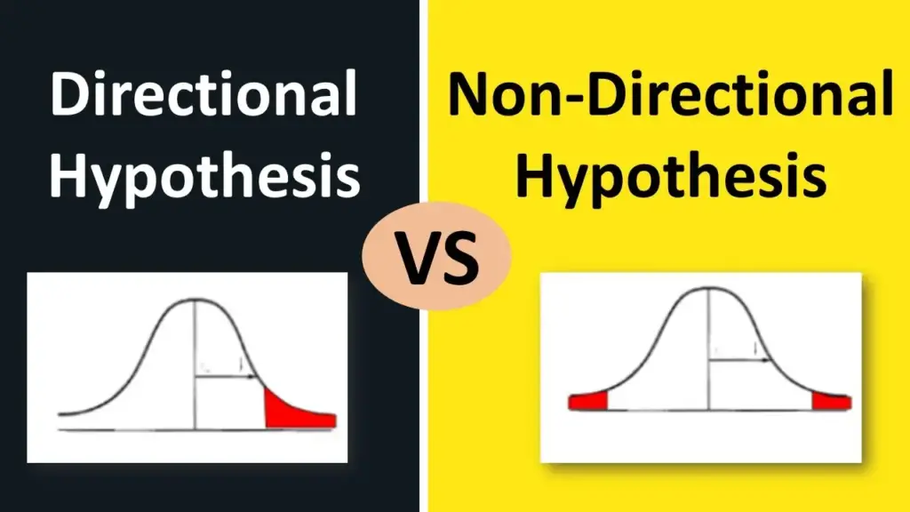
In the world of research and statistical analysis, formulating hypotheses is a crucial step in the scientific process. Hypotheses guide researchers in making predictions and testing relationships between variables. When it comes to hypotheses, there are two main types: directional and non-directional.

In this blog post, we will explore the differences between Directional vs. Non-Directional Hypothesis in Research and their implications in research.

Table of Contents

Directional Hypothesis

A directional hypothesis, also known as a one-tailed hypothesis, is formulated with a specific predicted direction of the relationship between variables. It indicates an expectation of the relationship being either positive or negative.

The directional hypothesis is often used when there is prior knowledge or theoretical reasoning supporting the predicted direction of the relationship. It allows researchers to make more specific predictions and draw conclusions based on the expected direction of the effect.

Example of Directional Hypothesis

For example, a directional hypothesis might state that “increased physical activity will lead to a decrease in body weight.” Here, the researcher expects a negative relationship between physical activity and body weight.

Advantages of Directional Hypothesis

Specific predictions: Directional hypotheses provide a clear prediction of the expected relationship between variables, allowing for a focused investigation.
Increased statistical power: By focusing on one direction of the relationship, researchers can allocate more statistical power to that specific direction, increasing the chances of detecting a significant effect if it exists.

Non-Directional Hypothesis

A non-directional hypothesis, also known as a two-tailed hypothesis, does not make a specific prediction about the direction of the relationship between variables. Instead, it states that there is a relationship, but without indicating whether it will be positive or negative.

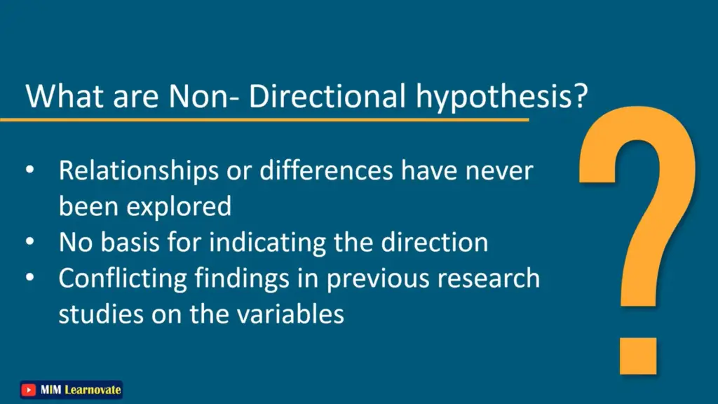
Non-directional hypotheses are often used when there is insufficient prior knowledge or theoretical basis to predict the direction of the relationship. It allows for a more exploratory approach, where the researcher is open to discovering the nature of the relationship through data analysis .

Read More: Internal Validity vs External Validity | Examples

Example of Non-Directional Hypothesis

For example, a non-directional hypothesis might state that “there is a relationship between caffeine consumption and reaction time.” Here, the researcher expects a relationship between the variables but does not specify the direction.

Read More: Population vs Sample | Examples

Advantages of Non-Directional Hypothesis:

Flexibility: Non-directional hypotheses provide flexibility in exploring relationships between variables without preconceived notions about the direction of the effect.
Open to unexpected findings : By not specifying the direction, researchers remain open to unexpected results or alternative explanations that may emerge during the analysis.

Difference Between Directional and Non-Directional Hypotheses

Choosing Between Directional and Non-Directional Hypotheses: The choice between a directional and non-directional hypothesis depends on the research question, existing knowledge, and theoretical background. Here are a few considerations for selecting the appropriate type of hypothesis:

Directional vs. Non-Directional Hypothesis

Prior research: If previous studies have established a clear direction of the relationship, a directional hypothesis may be more appropriate.
Theoretical reasoning: If there is a strong theoretical foundation supporting a specific direction, a directional hypothesis can provide a focused investigation.
Exploratory nature: If the research question is exploratory or lacks prior knowledge, a non-directional hypothesis allows for a more open-ended investigation.

Read More: Reliability vs Validity | Examples

Directional vs. Non-Directional Hypothesis

Formulating hypotheses is an essential step in the research process, guiding researchers in testing relationships between variables.

Directional hypotheses offer specific predictions about the expected direction of the relationship, whereas non-directional hypotheses allow for more exploratory investigations without preconceived notions of the direction.

The choice between these types of hypotheses depends on the research question, prior knowledge, and theoretical background.

By understanding the distinctions between directional and non-directional hypotheses, researchers can effectively formulate hypotheses that align with their research goals and contribute to the advancement of scientific knowledge.

Remember, hypotheses serve as a roadmap for research, and regardless of their type, they play a crucial role in scientific inquiry and the pursuit of knowledge.

Directional Hypothesis

A directional hypothesis is a one-tailed hypothesis that states the direction of the difference or relationship (e.g. boys are more helpful than girls).

Share on Facebook
Share on Twitter
Share by Email

Research Methods: MCQ Revision Test 1 for AQA A Level Psychology

Topic Videos

Example Answers for Research Methods: A Level Psychology, Paper 2, June 2018 (AQA)

Exam Support

Example Answer for Question 14 Paper 2: AS Psychology, June 2017 (AQA)

Model answer for question 11 paper 2: as psychology, june 2016 (aqa), a level psychology topic quiz - research methods.

Quizzes & Activities

Our subjects

› Criminology
› Economics
› Geography
› Health & Social Care
› Psychology
› Sociology
› Teaching & learning resources
› Student revision workshops
› Online student courses
› CPD for teachers
› Livestreams
› Teaching jobs

Boston House, 214 High Street, Boston Spa, West Yorkshire, LS23 6AD Tel: 01937 848885

› Contact us
› Terms of use
› Privacy & cookies

Research Writing and Analysis

NVivo Group and Study Sessions
SPSS This link opens in a new window
Statistical Analysis Group sessions
Using Qualtrics
Dissertation and Data Analysis Group Sessions
Defense Schedule - Commons Calendar This link opens in a new window
Research Process Flow Chart
Research Alignment Chapter 1 This link opens in a new window
Step 1: Seek Out Evidence
Step 2: Explain
Step 3: The Big Picture
Step 4: Own It
Step 5: Illustrate
Annotated Bibliography
Literature Review This link opens in a new window
Systematic Reviews & Meta-Analyses
How to Synthesize and Analyze
Synthesis and Analysis Practice
Synthesis and Analysis Group Sessions
Problem Statement
Purpose Statement
Conceptual Framework
Theoretical Framework
Quantitative Research Questions
Qualitative Research Questions
Trustworthiness of Qualitative Data
Analysis and Coding Example- Qualitative Data
Thematic Data Analysis in Qualitative Design
Dissertation to Journal Article This link opens in a new window
International Journal of Online Graduate Education (IJOGE) This link opens in a new window
Journal of Research in Innovative Teaching & Learning (JRIT&L) This link opens in a new window

Jump to DSE Guide

Purpose statement overview.

The purpose statement succinctly explains (on no more than 1 page) the objectives of the research study. These objectives must directly address the problem and help close the stated gap. Expressed as a formula:

Good purpose statements:

Flow from the problem statement and actually address the proposed problem
Are concise and clear
Answer the question ‘Why are you doing this research?’
Match the methodology (similar to research questions)
Have a ‘hook’ to get the reader’s attention
Set the stage by clearly stating, “The purpose of this (qualitative or quantitative) study is to ...

In PhD studies, the purpose usually involves applying a theory to solve the problem. In other words, the purpose tells the reader what the goal of the study is, and what your study will accomplish, through which theoretical lens. The purpose statement also includes brief information about direction, scope, and where the data will come from.

A problem and gap in combination can lead to different research objectives, and hence, different purpose statements. In the example from above where the problem was severe underrepresentation of female CEOs in Fortune 500 companies and the identified gap related to lack of research of male-dominated boards; one purpose might be to explore implicit biases in male-dominated boards through the lens of feminist theory. Another purpose may be to determine how board members rated female and male candidates on scales of competency, professionalism, and experience to predict which candidate will be selected for the CEO position. The first purpose may involve a qualitative ethnographic study in which the researcher observes board meetings and hiring interviews; the second may involve a quantitative regression analysis. The outcomes will be very different, so it’s important that you find out exactly how you want to address a problem and help close a gap!

The purpose of the study must not only align with the problem and address a gap; it must also align with the chosen research method. In fact, the DP/DM template requires you to name the research method at the very beginning of the purpose statement. The research verb must match the chosen method. In general, quantitative studies involve “closed-ended” research verbs such as determine , measure , correlate , explain , compare , validate , identify , or examine ; whereas qualitative studies involve “open-ended” research verbs such as explore , understand , narrate , articulate [meanings], discover , or develop .

A qualitative purpose statement following the color-coded problem statement (assumed here to be low well-being among financial sector employees) + gap (lack of research on followers of mid-level managers), might start like this:

In response to declining levels of employee well-being, the purpose of the qualitative phenomenology was to explore and understand the lived experiences related to the well-being of the followers of novice mid-level managers in the financial services industry. The levels of follower well-being have been shown to correlate to employee morale, turnover intention, and customer orientation (Eren et al., 2013). A combined framework of Leader-Member Exchange (LMX) Theory and the employee well-being concept informed the research questions and supported the inquiry, analysis, and interpretation of the experiences of followers of novice managers in the financial services industry.

A quantitative purpose statement for the same problem and gap might start like this:

In response to declining levels of employee well-being, the purpose of the quantitative correlational study was to determine which leadership factors predict employee well-being of the followers of novice mid-level managers in the financial services industry. Leadership factors were measured by the Leader-Member Exchange (LMX) assessment framework by Mantlekow (2015), and employee well-being was conceptualized as a compound variable consisting of self-reported turnover-intent and psychological test scores from the Mental Health Survey (MHS) developed by Johns Hopkins University researchers.

Both of these purpose statements reflect viable research strategies and both align with the problem and gap so it’s up to the researcher to design a study in a manner that reflects personal preferences and desired study outcomes. Note that the quantitative research purpose incorporates operationalized concepts or variables ; that reflect the way the researcher intends to measure the key concepts under study; whereas the qualitative purpose statement isn’t about translating the concepts under study as variables but instead aim to explore and understand the core research phenomenon.

Best Practices for Writing your Purpose Statement

Always keep in mind that the dissertation process is iterative, and your writing, over time, will be refined as clarity is gradually achieved. Most of the time, greater clarity for the purpose statement and other components of the Dissertation is the result of a growing understanding of the literature in the field. As you increasingly master the literature you will also increasingly clarify the purpose of your study.

The purpose statement should flow directly from the problem statement. There should be clear and obvious alignment between the two and that alignment will get tighter and more pronounced as your work progresses.

The purpose statement should specifically address the reason for conducting the study, with emphasis on the word specifically. There should not be any doubt in your readers’ minds as to the purpose of your study. To achieve this level of clarity you will need to also insure there is no doubt in your mind as to the purpose of your study.

Many researchers benefit from stopping your work during the research process when insight strikes you and write about it while it is still fresh in your mind. This can help you clarify all aspects of a dissertation, including clarifying its purpose.

Your Chair and your committee members can help you to clarify your study’s purpose so carefully attend to any feedback they offer.

The purpose statement should reflect the research questions and vice versa. The chain of alignment that began with the research problem description and continues on to the research purpose, research questions, and methodology must be respected at all times during dissertation development. You are to succinctly describe the overarching goal of the study that reflects the research questions. Each research question narrows and focuses the purpose statement. Conversely, the purpose statement encompasses all of the research questions.

Identify in the purpose statement the research method as quantitative, qualitative or mixed (i.e., “The purpose of this [qualitative/quantitative/mixed] study is to ...)

Avoid the use of the phrase “research study” since the two words together are redundant.

Follow the initial declaration of purpose with a brief overview of how, with what instruments/data, with whom and where (as applicable) the study will be conducted. Identify variables/constructs and/or phenomenon/concept/idea. Since this section is to be a concise paragraph, emphasis must be placed on the word brief. However, adding these details will give your readers a very clear picture of the purpose of your research.

Developing the purpose section of your dissertation is usually not achieved in a single flash of insight. The process involves a great deal of reading to find out what other scholars have done to address the research topic and problem you have identified. The purpose section of your dissertation could well be the most important paragraph you write during your academic career, and every word should be carefully selected. Think of it as the DNA of your dissertation. Everything else you write should emerge directly and clearly from your purpose statement. In turn, your purpose statement should emerge directly and clearly from your research problem description. It is good practice to print out your problem statement and purpose statement and keep them in front of you as you work on each part of your dissertation in order to insure alignment.

It is helpful to collect several dissertations similar to the one you envision creating. Extract the problem descriptions and purpose statements of other dissertation authors and compare them in order to sharpen your thinking about your own work. Comparing how other dissertation authors have handled the many challenges you are facing can be an invaluable exercise. Keep in mind that individual universities use their own tailored protocols for presenting key components of the dissertation so your review of these purpose statements should focus on content rather than form.

Once your purpose statement is set it must be consistently presented throughout the dissertation. This may require some recursive editing because the way you articulate your purpose may evolve as you work on various aspects of your dissertation. Whenever you make an adjustment to your purpose statement you should carefully follow up on the editing and conceptual ramifications throughout the entire document.

In establishing your purpose you should NOT advocate for a particular outcome. Research should be done to answer questions not prove a point. As a researcher, you are to inquire with an open mind, and even when you come to the work with clear assumptions, your job is to prove the validity of the conclusions reached. For example, you would not say the purpose of your research project is to demonstrate that there is a relationship between two variables. Such a statement presupposes you know the answer before your research is conducted and promotes or supports (advocates on behalf of) a particular outcome. A more appropriate purpose statement would be to examine or explore the relationship between two variables.

Your purpose statement should not imply that you are going to prove something. You may be surprised to learn that we cannot prove anything in scholarly research for two reasons. First, in quantitative analyses, statistical tests calculate the probability that something is true rather than establishing it as true. Second, in qualitative research, the study can only purport to describe what is occurring from the perspective of the participants. Whether or not the phenomenon they are describing is true in a larger context is not knowable. We cannot observe the phenomenon in all settings and in all circumstances.

Writing your Purpose Statement

It is important to distinguish in your mind the differences between the Problem Statement and Purpose Statement.

The Problem Statement is why I am doing the research

The Purpose Statement is what type of research I am doing to fit or address the problem

The Purpose Statement includes:

Method of Study
Specific Population

Remember, as you are contemplating what to include in your purpose statement and then when you are writing it, the purpose statement is a concise paragraph that describes the intent of the study, and it should flow directly from the problem statement. It should specifically address the reason for conducting the study, and reflect the research questions. Further, it should identify the research method as qualitative, quantitative, or mixed. Then provide a brief overview of how the study will be conducted, with what instruments/data collection methods, and with whom (subjects) and where (as applicable). Finally, you should identify variables/constructs and/or phenomenon/concept/idea.

Qualitative Purpose Statement

Creswell (2002) suggested for writing purpose statements in qualitative research include using deliberate phrasing to alert the reader to the purpose statement. Verbs that indicate what will take place in the research and the use of non-directional language that do not suggest an outcome are key. A purpose statement should focus on a single idea or concept, with a broad definition of the idea or concept. How the concept was investigated should also be included, as well as participants in the study and locations for the research to give the reader a sense of with whom and where the study took place.

Creswell (2003) advised the following script for purpose statements in qualitative research:

“The purpose of this qualitative_________________ (strategy of inquiry, such as ethnography, case study, or other type) study is (was? will be?) to ________________ (understand? describe? develop? discover?) the _________________(central phenomenon being studied) for ______________ (the participants, such as the individual, groups, organization) at __________(research site). At this stage in the research, the __________ (central phenomenon being studied) will be generally defined as ___________________ (provide a general definition)” (pg. 90).

Quantitative Purpose Statement

Creswell (2003) offers vast differences between the purpose statements written for qualitative research and those written for quantitative research, particularly with respect to language and the inclusion of variables. The comparison of variables is often a focus of quantitative research, with the variables distinguishable by either the temporal order or how they are measured. As with qualitative research purpose statements, Creswell (2003) recommends the use of deliberate language to alert the reader to the purpose of the study, but quantitative purpose statements also include the theory or conceptual framework guiding the study and the variables that are being studied and how they are related.

Creswell (2003) suggests the following script for drafting purpose statements in quantitative research:

“The purpose of this _____________________ (experiment? survey?) study is (was? will be?) to test the theory of _________________that _________________ (compares? relates?) the ___________(independent variable) to _________________________(dependent variable), controlling for _______________________ (control variables) for ___________________ (participants) at _________________________ (the research site). The independent variable(s) _____________________ will be generally defined as _______________________ (provide a general definition). The dependent variable(s) will be generally defined as _____________________ (provide a general definition), and the control and intervening variables(s), _________________ (identify the control and intervening variables) will be statistically controlled in this study” (pg. 97).

Sample Purpose Statements

The purpose of this qualitative study was to determine how participation in service-learning in an alternative school impacted students academically, civically, and personally. There is ample evidence demonstrating the failure of schools for students at-risk; however, there is still a need to demonstrate why these students are successful in non-traditional educational programs like the service-learning model used at TDS. This study was unique in that it examined one alternative school’s approach to service-learning in a setting where students not only serve, but faculty serve as volunteer teachers. The use of a constructivist approach in service-learning in an alternative school setting was examined in an effort to determine whether service-learning participation contributes positively to academic, personal, and civic gain for students, and to examine student and teacher views regarding the overall outcomes of service-learning. This study was completed using an ethnographic approach that included observations, content analysis, and interviews with teachers at The David School.
The purpose of this quantitative non-experimental cross-sectional linear multiple regression design was to investigate the relationship among early childhood teachers’ self-reported assessment of multicultural awareness as measured by responses from the Teacher Multicultural Attitude Survey (TMAS) and supervisors’ observed assessment of teachers’ multicultural competency skills as measured by the Multicultural Teaching Competency Scale (MTCS) survey. Demographic data such as number of multicultural training hours, years teaching in Dubai, curriculum program at current school, and age were also examined and their relationship to multicultural teaching competency. The study took place in the emirate of Dubai where there were 14,333 expatriate teachers employed in private schools (KHDA, 2013b).
The purpose of this quantitative, non-experimental study is to examine the degree to which stages of change, gender, acculturation level and trauma types predicts the reluctance of Arab refugees, aged 18 and over, in the Dearborn, MI area, to seek professional help for their mental health needs. This study will utilize four instruments to measure these variables: University of Rhode Island Change Assessment (URICA: DiClemente & Hughes, 1990); Cumulative Trauma Scale (Kira, 2012); Acculturation Rating Scale for Arabic Americans-II Arabic and English (ARSAA-IIA, ARSAA-IIE: Jadalla & Lee, 2013), and a demographic survey. This study will examine 1) the relationship between stages of change, gender, acculturation levels, and trauma types and Arab refugees’ help-seeking behavior, 2) the degree to which any of these variables can predict Arab refugee help-seeking behavior. Additionally, the outcome of this study could provide researchers and clinicians with a stage-based model, TTM, for measuring Arab refugees’ help-seeking behavior and lay a foundation for how TTM can help target the clinical needs of Arab refugees. Lastly, this attempt to apply the TTM model to Arab refugees’ condition could lay the foundation for future research to investigate the application of TTM to clinical work among refugee populations.
The purpose of this qualitative, phenomenological study is to describe the lived experiences of LLM for 10 EFL learners in rural Guatemala and to utilize that data to determine how it conforms to, or possibly challenges, current theoretical conceptions of LLM. In accordance with Morse’s (1994) suggestion that a phenomenological study should utilize at least six participants, this study utilized semi-structured interviews with 10 EFL learners to explore why and how they have experienced the motivation to learn English throughout their lives. The methodology of horizontalization was used to break the interview protocols into individual units of meaning before analyzing these units to extract the overarching themes (Moustakas, 1994). These themes were then interpreted into a detailed description of LLM as experienced by EFL students in this context. Finally, the resulting description was analyzed to discover how these learners’ lived experiences with LLM conformed with and/or diverged from current theories of LLM.
The purpose of this qualitative, embedded, multiple case study was to examine how both parent-child attachment relationships are impacted by the quality of the paternal and maternal caregiver-child interactions that occur throughout a maternal deployment, within the context of dual-military couples. In order to examine this phenomenon, an embedded, multiple case study was conducted, utilizing an attachment systems metatheory perspective. The study included four dual-military couples who experienced a maternal deployment to Operation Iraqi Freedom (OIF) or Operation Enduring Freedom (OEF) when they had at least one child between 8 weeks-old to 5 years-old. Each member of the couple participated in an individual, semi-structured interview with the researcher and completed the Parenting Relationship Questionnaire (PRQ). “The PRQ is designed to capture a parent’s perspective on the parent-child relationship” (Pearson, 2012, para. 1) and was used within the proposed study for this purpose. The PRQ was utilized to triangulate the data (Bekhet & Zauszniewski, 2012) as well as to provide some additional information on the parents’ perspective of the quality of the parent-child attachment relationship in regards to communication, discipline, parenting confidence, relationship satisfaction, and time spent together (Pearson, 2012). The researcher utilized the semi-structured interview to collect information regarding the parents' perspectives of the quality of their parental caregiver behaviors during the deployment cycle, the mother's parent-child interactions while deployed, the behavior of the child or children at time of reunification, and the strategies or behaviors the parents believe may have contributed to their child's behavior at the time of reunification. The results of this study may be utilized by the military, and by civilian providers, to develop proactive and preventive measures that both providers and parents can implement, to address any potential adverse effects on the parent-child attachment relationship, identified through the proposed study. The results of this study may also be utilized to further refine and understand the integration of attachment theory and systems theory, in both clinical and research settings, within the field of marriage and family therapy.

Was this resource helpful?

<< Previous: Problem Statement
Next: Conceptual Framework >>
Last Updated: May 16, 2024 8:25 AM
URL: https://resources.nu.edu/researchtools

Thank you for visiting nature.com. You are using a browser version with limited support for CSS. To obtain the best experience, we recommend you use a more up to date browser (or turn off compatibility mode in Internet Explorer). In the meantime, to ensure continued support, we are displaying the site without styles and JavaScript.

View all journals
My Account Login
Explore content
About the journal
Publish with us
Sign up for alerts
Open access
Published: 20 May 2024

Testing theory of mind in large language models and humans

James W. A. Strachan ORCID: orcid.org/0000-0002-8618-3834 1 ,
Dalila Albergo ORCID: orcid.org/0000-0002-8039-5414 2 , 3 ,
Giulia Borghini 2 ,
Oriana Pansardi ORCID: orcid.org/0000-0001-6092-1889 1 , 2 , 4 ,
Eugenio Scaliti ORCID: orcid.org/0000-0002-4977-2197 1 , 2 , 5 , 6 ,
Saurabh Gupta ORCID: orcid.org/0000-0001-6978-4243 7 ,
Krati Saxena ORCID: orcid.org/0000-0001-7049-9685 7 ,
Alessandro Rufo ORCID: orcid.org/0009-0003-8565-4192 7 ,
Stefano Panzeri ORCID: orcid.org/0000-0003-1700-8909 8 ,
Guido Manzi ORCID: orcid.org/0009-0009-2927-3380 7 ,
Michael S. A. Graziano 9 &
Cristina Becchio ORCID: orcid.org/0000-0002-6845-0521 1 , 2

Nature Human Behaviour ( 2024 ) Cite this article

Metrics details

Human behaviour

At the core of what defines us as humans is the concept of theory of mind: the ability to track other people’s mental states. The recent development of large language models (LLMs) such as ChatGPT has led to intense debate about the possibility that these models exhibit behaviour that is indistinguishable from human behaviour in theory of mind tasks. Here we compare human and LLM performance on a comprehensive battery of measurements that aim to measure different theory of mind abilities, from understanding false beliefs to interpreting indirect requests and recognizing irony and faux pas. We tested two families of LLMs (GPT and LLaMA2) repeatedly against these measures and compared their performance with those from a sample of 1,907 human participants. Across the battery of theory of mind tests, we found that GPT-4 models performed at, or even sometimes above, human levels at identifying indirect requests, false beliefs and misdirection, but struggled with detecting faux pas. Faux pas, however, was the only test where LLaMA2 outperformed humans. Follow-up manipulations of the belief likelihood revealed that the superiority of LLaMA2 was illusory, possibly reflecting a bias towards attributing ignorance. By contrast, the poor performance of GPT originated from a hyperconservative approach towards committing to conclusions rather than from a genuine failure of inference. These findings not only demonstrate that LLMs exhibit behaviour that is consistent with the outputs of mentalistic inference in humans but also highlight the importance of systematic testing to ensure a non-superficial comparison between human and artificial intelligences.

People care about what other people think and expend a lot of effort thinking about what is going on in other minds. Everyday life is full of social interactions that only make sense when considered in light of our capacity to represent other minds: when you are standing near a closed window and a friend says, ‘It’s a bit hot in here’, it is your ability to think about her beliefs and desires that allows you to recognize that she is not just commenting on the temperature but politely asking you to open the window 1 .

This ability for tracking other people’s mental states is known as theory of mind. Theory of mind is central to human social interactions—from communication to empathy to social decision-making—and has long been of interest to developmental, social and clinical psychologists. Far from being a unitary construct, theory of mind refers to an interconnected set of notions that are combined to explain, predict, and justify the behaviour of others 2 . Since the term ‘theory of mind’ was first introduced in 1978 (ref. 3 ), dozens of tasks have been developed to study it, including indirect measures of belief attribution using reaction times 4 , 5 , 6 and looking or searching behaviour 7 , 8 , 9 , tasks examining the ability to infer mental states from photographs of eyes 10 , and language-based tasks assessing false belief understanding 11 , 12 and pragmatic language comprehension 13 , 14 , 15 , 16 . These measures are proposed to test early, efficient but inflexible implicit processes as well as later-developing, flexible and demanding explicit abilities that are crucial for the generation and comprehension of complex behavioural interactions 17 , 18 involving phenomena such as misdirection, irony, implicature and deception.

The recent rise of large language models (LLMs), such as generative pre-trained transformer (GPT) models, has shown some promise that artificial theory of mind may not be too distant an idea. Generative LLMs exhibit performance that is characteristic of sophisticated decision-making and reasoning abilities 19 , 20 including solving tasks widely used to test theory of mind in humans 21 , 22 , 23 , 24 . However, the mixed success of these models 23 , along with their vulnerability to small perturbations to the provided prompts, including simple changes in characters’ perceptual access 25 , raises concerns about the robustness and interpretability of the observed successes. Even in cases where these models are capable of solving complex tasks 20 that are cognitively demanding even for human adults 17 , it cannot be taken for granted that they will not be tripped up by a simpler task that a human would find trivial 26 . As a result, work in LLMs has begun to question whether these models rely on shallow heuristics rather than robust performance that parallels human theory of mind abilities 27 .

In the service of the broader multidisciplinary study of machine behaviour 28 , there have been recent calls for a ‘machine psychology’ 29 that have argued for using tools and paradigms from experimental psychology to systematically investigate the capacities and limits of LLMs 30 . A systematic experimental approach to studying theory of mind in LLMs involves using a diverse set of theory of mind measures, delivering multiple repetitions of each test, and having clearly defined benchmarks of human performance against which to compare 31 . In this Article, we adopt such an approach to test the performance of LLMs in a wide range of theory of mind tasks. We tested the chat-enabled version of GPT-4, the latest LLM in the GPT family of models, and its predecessor ChatGPT-3.5 (hereafter GPT-3.5) in a comprehensive set of psychological tests spanning different theory of mind abilities, from those that are less cognitively demanding for humans such as understanding indirect requests to more cognitively demanding abilities such as recognizing and articulating complex mental states like misdirection or irony 17 . GPT models are closed, evolving systems. In the interest of reproducibility 32 , we also tested the open-weight LLaMA2-Chat models on the same tests. To understand the variability and boundary limitations of LLMs’ social reasoning capacities, we exposed each model to multiple repetitions of each test across independent sessions and compared their performance with that of a sample of human participants (total N = 1,907). Using variants of the tests considered, we were able to examine the processes behind the models’ successes and failures in these tests.

Theory of mind battery

We selected a set of well-established theory of mind tests spanning different abilities: the hinting task 14 , the false belief task 11 , 33 , the recognition of faux pas 13 , and the strange stories 15 , 16 . We also included a test of irony comprehension using stimuli adapted from a previous study 34 . Each test was administered separately to GPT-4, GPT-3.5 and LLaMA2-70B-Chat (hereafter LLaMA2-70B) across 15 chats. We also tested two other sizes of LLaMA2 model (7B and 13B), the results of which are reported in Supplementary Information section 1 . Because each chat is a separate and independent session, and information about previous sessions is not retained, this allowed us to treat each chat (session) as an independent observation. Responses were scored in accordance with the scoring protocols for each test in humans ( Methods ) and compared with those collected from a sample of 250 human participants. Tests were administered by presenting each item sequentially in a written format that ensured a species-fair comparison 35 ( Methods ) between LLMs and human participants.

Performance across theory of mind tests

Except for the irony test, all other tests in our battery are publicly available tests accessible within open databases and scholarly journal articles. To ensure that models did not merely replicate training set data, we generated novel items for each published test ( Methods ). These novel test items matched the logic of the original test items but used a different semantic content. The text of original and novel items and the coded responses are available on the OSF (methods and resource availability).

Figure 1a compares the performance of LLMs against the performance of human participants across all tests included in the battery. Differences in performance on original items versus novel items, separately for each test and model, are shown in Fig. 1b .

a , Original test items for each test showing the distribution of test scores for individual sessions and participants. Coloured dots show the average response score across all test items for each individual test session (LLMs) or participant (humans). Black dots indicate the median for each condition. P values were computed from Holm-corrected Wilcoxon two-way tests comparing LLM scores ( n = 15 LLM observations) against human scores (irony, N = 50 human participants; faux pas, N = 51 human participants; hinting, N = 48 human participants; strange stories, N = 50 human participants). Tests are ordered in descending order of human performance. b , Interquartile ranges of the average scores on the original published items (dark colours) and novel items (pale colours) across each test (for LLMs, n = 15 LLM observations; for humans, false belief, N = 49 human participants; faux pas, N = 51 human participants; hinting, N = 48 human participants; strange stories, N = 50 human participants). Empty diamonds indicate the median scores, and filled circles indicate the upper and lower bounds of the interquartile range. P values shown are from Holm-corrected Wilcoxon two-way tests comparing performance on original items against the novel items generated as controls for this study.

Source data

False belief.

Both human participants and LLMs performed at ceiling on this test (Fig. 1a ). All LLMs correctly reported that an agent who left the room while the object was moved would later look for the object in the place where they remembered seeing it, even though it no longer matched the current location. Performance on novel items was also near perfect (Fig. 1b ), with only 5 human participants out of 51 making one error, typically by failing to specify one of the two locations (for example, ‘He’ll look in the room’; Supplementary Information section 2 ).

In humans, success on the false belief task requires inhibiting one’s own belief about reality in order to use one’s knowledge about the character’s mental state to derive predictions about their behaviour. However, with LLMs, performance may be explained by lower-level explanations than belief tracking 27 . Supporting this interpretation, LLMs such as ChatGPT have been shown to be susceptible to minor alterations to the false belief formulation 25 , 27 , such as making the containers where the object is hidden transparent or asking about the belief of the character who moved the object rather than the one who was out of the room. Such perturbations of the standard false belief structure are assumed not to matter for humans (who possess a theory of mind) 25 . In a control study using these perturbation variants (Supplementary Information section 4 and Supplementary Appendix 1 ), we replicated the poor performance of GPT models found in previous studies 25 . However, we found that human participants ( N = 757) also failed on half of these perturbations. Understanding these failures and the similarities and differences in how humans and LLMs may arrive at the same outcome requires further systematic investigation. For example, because these perturbations also involve changes in the physical properties of the environment, it is difficult to establish whether LLMs (and humans) failed because they were sticking to the familiar script and were unable to automatically attribute an updated belief, or because they did not consider physical principles (for example, transparency).

GPT-4 performed significantly better than human levels ( Z = 0.00, P = 0.040, r = 0.32, 95% confidence interval (CI) 0.14–0.48). By contrast, both GPT-3.5 ( Z = −0.17, P = 2.37 × 10 −6 , r = 0.64, 95% CI 0.49–0.77) and LLaMA2-70B ( Z = −0.42, P = 2.39 × 10 −7 , r = 0.70, 95% CI 0.55–0.79) performed below human levels (Fig. 1a ). GPT-3.5 performed perfectly at recognizing non-ironic control statements but made errors at recognizing ironic utterances (Supplementary Information section 2 ). Control analysis revealed a significant order effect, whereby GPT-3.5 made more errors on earlier trials than later ones (Supplementary Information section 3 ). LLaMA2-70B made errors when recognizing both ironic and non-ironic control statements, suggesting an overall poor discrimination of irony.

On this test, GPT-4 scored notably lower than human levels ( Z = −0.40, P = 5.42 × 10 −5 , r = 0.55, 95% CI 0.33–0.71) with isolated ceiling effects on specific items (Supplementary Information section 2 ). GPT-3.5 scored even worse, with its performance nearly at floor ( Z = −0.80, P = 5.95 × 10 −8 , r = 0.72, 95% CI 0.58–0.81) on all items except one. By contrast, LLaMA2-70B outperformed humans ( Z = 0.10, P = 0.002, r = 0.44, 95% CI 0.24–0.61) achieving 100% accuracy in all but one run.

The pattern of results for novel items was qualitatively similar (Fig. 1b ). Compared with original items, the novel items proved slightly easier for humans ( Z = −0.10, P = 0.029, r = 0.29, 95% CI 0.10–0.50) and more difficult for GPT-3.5 ( Z = 0.10, P = 0.002, r = 0.69, 95% CI 0.49–0.88), but not for GPT-4 and LLaMA2-70B ( P > 0.462; Bayes factor (BF 10 ) of 0.77 and 0.43, respectively). Given the poor performance of GPT-3.5 of the original test items, this difference was unlikely to be explained by a prior familiarity with the original items. These results were robust to alternative coding schemes (Supplementary Information section 5 ).

On this test, GPT-4 performance was significantly better than humans ( Z = 0.00, P = 0.040, r = 0.32, 95% CI 0.12–0.50). GPT-3.5 performance did not significantly differ from human performance ( Z = 0.00, P = 0.626, r = 0.06, 95% CI 0.01–0.33, BF 10 0.33). Only LLaMA2-70B scored significantly below human levels of performance on this test ( Z = −0.20, P = 5.42 × 10 −5 , r = 0.57, 95% CI 0.41–0.72).

Novel items proved easier than original items for both humans ( Z = −0.10, P = 0.008, r = 0.34, 95% CI 0.14–0.53) and LLaMA2-70B ( Z = −0.20, P = 9.18 × 10 −4 , r = 0.73, 95% CI 0.50–0.87) (Fig. 1b ). Scores on novel items did not differ from the original test items for GPT-3.5 ( Z = −0.03, P = 0.955, r = 0.24, 95% CI 0.02–0.59, BF 10 0.61) or GPT-4 ( Z = −0.10, P = 0.123, r = 0.44, 95% CI 0.07–0.75, BF 10 0.91). Given that better performance on novel items is the opposite of what a prior familiarity explanation would predict, it is likely that this difference for LLaMA2-70B was driven by differences in item difficulty.

Strange stories

GPT-4 significantly outperformed humans on this test ( Z = 0.13, P = 1.04 × 10 −5 , r = 0.60, 95% CI 0.46–0.72). The performance of GPT-3.5 did not significantly differ from humans ( Z = −0.06, P = 0.110, r = 0.24, 95% CI 0.03–0.44, BF 10 0.47), while LLaMA2-70B scored significantly lower than humans ( Z = −0.13, P = 0.005, r = 0.41, 95% CI 0.24–0.60). There were no differences between original and novel items for any model (all P > 0.085; BF 10 : human 0.22, GPT-3.5 1.46, LLaMA2-70B 0.46; the variance for GPT-4 was too low to compute a Bayes factor). As reported in Supplementary Information section 6 , partial successes were infrequent and more likely for LLaMA2-70B than for other models.

Understanding faux pas

In line with previous findings that GPT models struggle with faux pas 36 , in our battery, faux pas was the only test in which GPT-4 did not match or exceed human performance. Surprisingly, faux pas was also the only test in which LLaMA2-70B, which was otherwise the poorest-performing model, scored better than humans (Fig. 1 ).

The faux pas test consists of vignettes describing an interaction where one character (the speaker) says something they should not have said, not knowing or not realizing that they should not say it. To understand that a faux pas has occurred, one must represent two mental states: that the speaker does not know that they should not say what they said, and that the person hearing it (the victim) would feel insulted or hurt by what was said. Consider the following example of a story describing a faux pas:

Jill had just moved into a new house. She went shopping with her Mum and bought some new curtains. When Jill had just put them up, her best friend Lisa came round and said, "Oh, those curtains are horrible, I hope you're going to get some new ones." Jill asked, "Do you like the rest of my bedroom?"

Following the presentation of the story, four comprehension questions are asked. The first question is, ‘In the story, did somebody say something they should not have said?’ to which the correct answer is always yes. The second question asks the respondent to report what the person said that they should not have said, and the third question is a comprehension question specific to the content of the story. The fourth and key question, which was our focus for coding, relates to the speaker’s belief when they made the inappropriate utterance: ‘Did [Lisa] know that [the curtains were new]?’ The correct answer to this final question is always no.

Both GPT-4 and GPT-3.5 correctly identified that the victim would feel insulted or hurt, sometimes going so far as to provide additional details about why the utterance might cause offence. However, when asked whether the speaker was aware of the context that made their statement offensive (such as Lisa knowing that Jill had just bought the curtains), they failed to produce a correct answer. A closer look revealed that the overwhelming majority of the errors on this question reported that there was not enough information provided to be sure, for example:

Did Lisa know the curtains were new? GPT-4: […] It is unclear from the story whether Lisa knew the curtains were new or not.

Only two responses out of 349 reported that, yes, the character did know. We consider three alternative hypotheses for why GPT models, and specifically GPT-4, fail to answer this question correctly.

The first hypothesis, which we term the failure of inference hypothesis, is that models fail to generate inferences about the mental state of the speaker (note that we refer to inference here not in the sense of the processes by which biological organisms infer hidden states from their environment, but rather as any process of reasoning whereby conclusions are derived from a set of propositional premises). Recognizing a faux pas in this test relies on contextual information beyond that encoded within the story (for example, about social norms). For example, in the above example there is no information in the story to indicate that saying that the newly bought curtains are horrible is inappropriate, but this is a necessary proposition that must be accepted in order to accurately infer the mental states of the characters. This inability to use non-embedded information would fundamentally impair the ability of GPT-4 to compute inferences.

The second hypothesis, which we term the Buridan’s ass hypothesis, is that models are capable of inferring mental states but cannot choose between them, as with the eponymous rational agent caught between two equally appetitive bales of hay that starves because it cannot resolve the paradox of making a decision in the absence of a clear preference 37 . Under this hypothesis, GPT models can propose the correct answer (a faux pas) as one among several possible alternatives but do not rank these alternatives in terms of likelihood. In partial support of this hypothesis, responses from both GPT models occasionally indicate that the speaker may not know or remember but present this as one hypothesis among alternatives (Supplementary Information section 5 ).

The third hypothesis, which we term the hyperconservatism hypothesis, is that GPT models are able both to compute inferences about the mental states of characters and recognise a false belief or lack of knowledge as the likeliest explanation among competing alternatives but refrain from committing to a single explanation out of an excess of caution. GPT models are powerful language generators, but they are also subject to inhibitory mitigation processes 38 . It is possible that such processes could lead to an overly conservative stance where GPT models do not commit to the likeliest explanation despite being able to generate it.

To differentiate between these hypotheses, we devised a variant of the faux pas test where the question assessing performance on the faux pas test was formulated in terms of likelihood (hereafter, the faux pas likelihood test). Specifically, rather than ask whether the speaker knew or did not know, we asked whether it was more likely that the speaker knew or did not know. Under the hyperconservatism hypothesis, GPT models should be able to both make the inference that the speaker did not know and identify it as more likely among alternatives, and so we would expect the models to respond accurately that it was more likely that the speaker did not know. In case of uncertainty or incorrect responses, we further prompted models to describe the most likely explanation. Under the Buridan’s ass hypothesis, we expected this question would elicit multiple alternative explanations that would be presented as equally plausible, while under the failure of inference hypothesis, we expected that GPT would not be able to generate the right answer at all as a plausible explanation.

As shown in Fig. 2a , on the faux pas likelihood test GPT-4 demonstrated perfect performance, with all responses identifying without any prompting that it was more likely that the speaker did not know the context. GPT-3.5 also showed improved performance, although it did require prompting in a few instances (~3% of items) and occasionally failed to recognize the faux pas (~9% of items; see Supplementary Information section 7 for a qualitative analysis of response types).

a , Scores of the two GPT models on the original framing of the faux pas question (‘Did they know…?’) and the likelihood framing (‘Is it more likely that they knew or didn’t know…?’). Dots show average score across trials ( n = 15 LLM observations) on particular items to allow comparison between the original faux pas test and the new faux pas likelihood test. Halfeye plots show distributions, medians (black points), 66% (thick grey lines) and 99% quantiles (thin grey lines) of the response scores on different items ( n = 15 different stories involving faux pas). b , Response scores to three variants of the faux pas test: faux pas (pink), neutral (grey) and knowledge-implied variants (teal). Responses were coded as categorical data as ‘didn’t know’, ‘unsure’ or ‘knew’ and assigned a numerical coding of −1, 0 and +1. Filled balloons are shown for each model and variant, and the size of each balloon indicates the count frequency, which was the categorical data used to compute chi-square tests. Bars show the direction bias score computed as the average across responses of the categorical data coded as above. On the right of the plot, P values (one-sided) of Holm-corrected chi-square tests are shown comparing the distribution of response type frequencies in the faux pas and knowledge-implied variants against neutral.

Taken together, these results support the hyperconservatism hypothesis, as they indicate that GPT-4, and to a lesser but still notable extent GPT-3.5, successfully generated inferences about the mental states of the speaker and identified that an unintentional offence was more likely than an intentional insult. Thus, failure to respond correctly to the original phrasing of the question does not reflect a failure of inference, nor indecision among alternatives the model considered equally plausible, but an overly conservative approach that prevented commitment to the most likely explanation.

Testing information integration

A potential confound of the above results is that, as the faux pas test includes only items where a faux pas occurs, any model biased towards attributing ignorance would demonstrate perfect performance without having to integrate the information provided by the story. This potential bias could explain the perfect performance of LLaMA2-70B in the original faux pas test (where the correct answer is always, ‘no’) as well as GPT-4’s perfect and GPT-3.5’s good performance on the faux pas likelihood test (where the correct answer is always ‘more likely that they didn’t know’).

To control for this, we developed a novel set of variants of the faux pas likelihood test manipulating the likelihood that the speaker knew or did not know (hereafter the belief likelihood test). For each test item, all newly generated for this control study, we created three variants: a ‘faux pas’ variant, a ‘neutral’ variant, and a ‘knowledge-implied’ variant ( Methods ). In the faux pas variant, the utterance suggested that the speaker did not know the context. In the neutral variant, the utterance suggested neither that they knew nor did not know. In the knowledge-implied variant, the utterance suggested that the speaker knew (for the full text of all items, see Supplementary Appendix 2 ).

If the models’ responses reflect a true discrimination of the relative likelihood of the two explanations (that the person knew versus that they didn’t know, hereafter ‘knew’ and ‘didn’t know’), then the distribution of ‘knew’ and ‘didn’t know’ responses should be different across variants. Specifically, relative to the neutral variant, ‘didn’t know’ responses should predominate for the faux pas, and ‘knew’ responses should predominate for the knowledge-implied variant. If the responses of the models do not discriminate between the three variants, or discriminate only partially, then it is likely that responses are affected by a bias or heuristic unrelated to the story content.

We adapted the three variants (faux pas, neutral and knowledge implied) for six stories, administering each test item separately to each LLM and a new sample of human participants (total N = 900). Responses were coded using a numeric code to indicate which, if either, of the knew/didn’t know explanations the response endorsed (−1, didn’t know; 0, unsure or impossible to tell; +1, knew). These coded scores were then averaged for each story to give a directional score for each variant such that negative values indicated the model was more likely to endorse the ‘didn’t know’ explanation, while positive values indicated the model was more likely to endorse the ‘knew’ explanation. These results are shown in Fig. 2b . As expected, humans were more likely to report that the speaker did not know for faux pas than for neutral ( χ 2 (2) = 56.20, P = 3.82 × 10 −12 ) and more likely to report that the speaker did know for knowledge implied than for neutral ( χ 2 (2) = 143, P = 6.60 × 10 −31 ). Humans also reported uncertainty on a small proportion of trials, with a higher proportion in the neutral condition (28 out of 303 responses) than in the other variants (11 out of 303 for faux pas, and 0 out of 298 for knowledge implied).

Similarly to humans, GPT-4 was more likely to endorse the ‘didn’t know’ explanation for faux pas than for neutral ( χ 2 (2) = 109, P = 1.54 × 10 −23 ) and more likely to endorse the ‘knew’ explanation for knowledge implied than for neutral ( χ 2 (2) = 18.10, P = 3.57 × 10 −4 ). GPT-4 was also more likely to report uncertainty in the neutral condition than responding randomly (42 out of 90 responses, versus 6 and 17 in the faux pas and knowledge-implied variants, respectively).

The pattern of responses for GPT-3.5 was similar, with the model being more likely to report that the speaker didn’t know for faux pas than for neutral ( χ 2 (1) = 8.44, P = 0.007) and more likely that the character knew for knowledge implied than for neutral ( χ 2 (1) = 21.50, P = 1.82 × 10 −5 ). Unlike GPT-4, GPT-3.5 never reported uncertainty in response to any variants and always selected one of the two explanations as the likelier even in the neutral condition.

LLaMA2-70B was also more likely to report that the speaker didn’t know in response to faux pas than neutral ( χ 2 (1) = 20.20, P = 2.81 × 10 −5 ), which was consistent with this model’s ceiling performance in the original formulation of the test. However, it showed no differentiation between neutral and knowledge implied ( χ 2 (1) = 1.80, P = 0.180, BF 10 0.56). As with GPT-3.5, LLaMA2-70B never reported uncertainty in response to any variants and always selected one of the two explanations as the likelier.

Furthermore, the responses of LLaMA2-70B and, to a lesser extent, GPT-3.5 appeared to be subject to a response bias towards affirming that someone had said something they should not have said. Although the responses to the first question (which involved recognising that there was an offensive remark made) were of secondary interest to our study, it was notable that, although all models could correctly identify that an offensive remark had been made in the faux pas condition (all LLMs 100%, humans 83.61%), only GPT-4 reliably reported that there was no offensive statement in the neutral and knowledge-implied conditions (15.47% and 27.78%, respectively), with similar proportions to human responses (neutral 19.27%, knowledge implied 30.10%). GPT-3.5 was more likely to report that somebody made an offensive remark in all conditions (neutral 71.11%, knowledge implied 87.78%), and LLaMA2-70B always reported that somebody in the story had made an offensive remark.

We collated a battery of tests to comprehensively measure performance in theory of mind tasks in three LLMs (GPT-4, GPT-3.5 and LLaMA2-70B) and compared these against the performance of a large sample of human participants. Our findings validate the methodological approach taken in this study using a battery of multiple tests spanning theory of mind abilities, exposing language models to multiple sessions and variations in both structure and content, and implementing procedures to ensure a fair, non-superficial comparison between humans and machines 35 . This approach enabled us to reveal the existence of specific deviations from human-like behaviour that would have remained hidden using a single theory of mind test, or a single run of each test.

Both GPT models exhibited impressive performance in tasks involving beliefs, intentions and non-literal utterances, with GPT-4 exceeding human levels in the irony, hinting and strange stories. Both GPT-4 and GPT-3.5 failed only on the faux pas test. Conversely, LLaMA2-70B, which was otherwise the poorest-performing model, outperformed humans on the faux pas. Understanding a faux pas involves two aspects: recognizing that one person (the victim) feels insulted or upset and understanding that another person (the speaker) holds a mistaken belief or lacks some relevant knowledge. To examine the nature of models’ successes and failures on this test, we developed and tested new variants of the faux pas test in a set of control experiments.

Our first control experiment using a likelihood framing of the belief question (faux pas likelihood test), showed that GPT-4, and to a lesser extent GPT-3.5, correctly identified the mental state of both the victim and the speaker and selected as the most likely explanation the speaker not knowing or remembering the relevant knowledge that made their statement inappropriate. Despite this, both models consistently provided an incorrect response (at least when compared against human responses) when asked whether the speaker knew or remembered this knowledge, responding that there was insufficient information provided. In line with the hyperconservatism hypothesis, these findings imply that, while GPT models can identify unintentional offence as the most likely explanation, their default responses do not commit to this explanation. This finding is consistent with longitudinal evidence that GPT models have become more reluctant to answer opinion questions over time 39 .

Further supporting that the failures of GPT at recognizing faux pas were due to hyperconservatism in answering the belief question rather than a failure of inference, a second experiment using the belief likelihood test showed that GPT responses integrated information in the story to accurately interpret the speaker’s mental state. When the utterance suggested that the speaker knew, GPT responses acknowledged the higher likelihood of the ‘knew’ explanation. LLaMA2-70B, on the other hand, did not differentiate between scenarios where the speaker was implied to know and when there was no information one way or another, raising the concern that the perfect performance of LLaMA2-70B on this task may be illusory.

The pattern of failures and successes of GPT models on the faux pas test and its variants may be the result of their underlying architecture. In addition to transformers (generative algorithms that produce text output), GPT models also include mitigation measures to improve factuality and avoid users’ overreliance on them as sources 38 . These measures include training to reduce hallucinations, the propensity of GPT models to produce nonsensical content or fabricate details that are not true in relation to the provided content. Failure on the faux pas test may be an exercise of caution driven by these mitigation measures, as passing the test requires committing to an explanation that lacks full evidence. This caution can also explain differences between tasks: both the faux pas and hinting tests require speculation to generate correct answers from incomplete information. However, while the hinting task allows for open-ended generation of text in ways to which LLMs are well suited, answering the faux pas test requires going beyond this speculation in order to commit to a conclusion.

The cautionary epistemic policy guiding the responses of GPT models introduces a fundamental difference in the way that humans and GPT models respond to social uncertainty 40 . In humans, thinking is, first and last, for the sake of doing 41 , 42 . Humans generally find uncertainty in social environments to be aversive and will incur additional costs to reduce it 43 . Theory of mind is crucial in reducing such uncertainty; the ability to reason about mental states—in combination with information about context, past experience and knowledge of social norms—helps individual reduce uncertainty and commit to likely hypotheses, allowing for successful navigation of the social environment as active agents 44 , 45 . GPT models, on the other hand, respond conservatively despite having access to tools to reduce uncertainty. The dissociation we describe between speculative reasoning and commitment mirrors recent evidence that, while GPT models demonstrate sophisticated and accurate performance in reasoning tasks about belief states, they struggle to translate this reasoning into strategic decisions and actions 46 .

These findings highlight a dissociation between competence and performance 35 , suggesting that GPT models may be competent, that is, have the technical sophistication to compute mentalistic-like inferences but perform differently from humans under uncertain circumstances as they do not compute these inferences spontaneously to reduce uncertainty. Such a distinction can be difficult to capture with quantitative approaches that code only for target response features, as machine failures and successes are the result of non-human-like processes 30 (see Supplementary Information section 7 for a preliminary qualitative breakdown of how GPT models’ successes on the new version of the faux pas test may not necessarily reflect perfect or human-like reasoning).

While LLMs are designed to emulate human-like responses, this does not mean that this analogy extends to the underlying cognition giving rise to those responses 47 . In this context, our findings imply a difference in how humans and GPT models trade off the costs associated with social uncertainty against the costs associated with prolonged deliberation 48 . This difference is perhaps not surprising considering that resolving uncertainty is a priority for brains adapted to deal with embodied decisions, such as deciding whether to approach or avoid, fight or flight, or cooperate or defect. GPT models and other LLMs do not operate within an environment and are not subject to the processing constraints that biological agents face to resolve competition between action choices, so may have limited advantages in narrowing the future prediction space 46 , 49 , 50 .

The dis-embodied cognition of GPT models could explain failures in recognizing faux pas, but they may also underlie their success on other tests. One example is the false belief test, one of the most widely used tools so far for testing the performance of LLMs on social cognitive tasks 19 , 21 , 22 , 23 , 25 , 51 , 52 . In this test, participants are presented with a story where a character’s belief about the world (the location of the item) differs from the participant’s own belief. The challenge in these stories is not remembering where the character last saw the item but rather in reconciling the incongruence between conflicting mental states. This is challenging for humans, who have their own perspective, their own sense of self and their own ability to track out-of-sight objects. However, if a machine does not have its own self-perspective because it is not subject to the constraints of navigating a body through an environment, as with GPT 53 , then tracking the belief of a character in a story does not pose the same challenge.

An important direction for future research will be to examine the impact of these non-human decision behaviours on second-person, real-time human–machine interactions 54 , 55 . Failure of commitment by GPT models, for example, may lead to negative affect in human conversational partners. However, it may also foster curiosity 40 . Understanding how GPTs’ performance on mentalistic inferences (or their absences) influences human social cognition in dynamically unfolding social interactions is an open challenge for future work.

The LLM landscape is fast-moving. Our findings highlight the importance of systematic testing and proper validation in human samples as a necessary foundation. As artificial intelligence (AI) continues to evolve, it also becomes increasingly important to heed calls for open science and open access to these models 32 . Direct access to the parameters, data and documentation used to construct models can allow for targeted probing and experimentation into the key parameters affecting social reasoning, informed by and building on comparisons with human data. As such, open models can not only serve to accelerate the development of future AI technologies but also serve as models of human cognition.

Ethical compliance

The research was approved by the local ethical committee (ASL 3 Genovese; protocol no. 192REG2015) and was carried out in accordance with the principles of the revised Helsinki Declaration.

Experimental model details

We tested two versions of OpenAI’s GPT: version 3.5, which was the default model at the time of testing, and version 4, which was the state-of-the-art model with enhanced reasoning, creativity and comprehension relative to previous models ( https://chat.openai.com/ ). Each test was delivered in a separate chat: GPT is capable of learning within a chat session, as it can remember both its own and the user’s previous messages to adapt its responses accordingly, but it does not retain this memory across new chats. As such, each new iteration of a test may be considered a blank slate with a new naive participant. The dates of data collection for the different stages are reported in Table 1 .

Three LLaMA2-Chat models were tested. These models were trained on sets of different sizes: 70, 13 and 7 billion tokens. All LLaMA2-Chat responses were collected using set parameters with the prompt, ‘You are a helpful AI assistant’, a temperature of 0.7, the maximum number of new tokens set at 512, a repetition penalty of 1.1, and a Top P of 0.9. Langchain’s conversation chain was used to create a memory context within individual chat sessions. Responses from all LLaMA2-Chat models were found to include a number of non-codable responses (for example, repeating the question without answering it), and these were regenerated individually and included with the full response set. For the 70B model, these non-responses were rare, but for the 13B and 7B models they were common enough to cause concern about the quality of these data. As such, only the responses of the 70B model are reported in the main manuscript and a comparison of this model against the smaller two is reported in Supplementary Information section 1 . Details and dates of data collection are reported in Table 1 .

For each test, we collected 15 sessions for each LLM. A session involved delivering all items of a single test within the same chat window. GPT-4 was subject to a 25-message limit per 3 h; to minimize interference, a single experimenter delivered all tests for GPT-4, while four other experimenters shared the duty of collecting responses from GPT-3.5.

Human participants were recruited online through the Prolific platform and the study was hosted on SoSci. We recruited native English speakers between the ages of 18 and 70 years with no history of psychiatric conditions and no history of dyslexia in particular. Further demographic data were not collected. We aimed to collect around 50 participants per test (theory of mind battery) or item (belief likelihood test, false belief perturbations). Thirteen participants who appeared to have generated their answers using LLMs or whose responses did not answer the questions were excluded. The final human sample was N = 1,907 (Table 1 ). All participants provided informed consent through the online survey and received monetary compensation in return for their participation at a rate of GBP£12 h −1 .

We selected a series of tests typically used in evaluating theory of mind capacity in human participants.

False belief assess the ability to infer that another person possesses knowledge that differs from the participant’s own (true) knowledge of the world. These tests consist of test items that follow a particular structure: character A and character B are together, character A deposits an item inside a hidden location (for example, a box), character A leaves, character B moves the item to a second hidden location (for example, a cupboard) and then character A returns. The question asked to the participant is: when character A returns, will they look for the item in the new location (where it truly is, matching the participant’s true belief) or the old location (where it was, matching character A’s false belief)?

In addition to the false belief condition, the test also uses a true belief control condition, where rather than move the item that character A hid, character B moves a different item to a new location. This is important for interpreting failures of false belief attribution as they ensure that any failures are not due to a recency effect (referring to the last location reported) but instead reflect an accurate belief tracking.

We adapted four false/true belief scenarios from the sandbox task used by Bernstein 33 and generated three novel items, each with false and true belief versions. These novel items followed the same structure as the original published items but with different details such as names, locations or objects to control for familiarity with the text of published items. Two story lists (false belief A, false belief B) were generated for this test such that each story only appeared once within a testing session and alternated between false and true belief depending on the session. In addition to the standard false/true belief scenarios, two additional catch stories were tested that involved minor alterations to the story structure. The results of these items are not reported here as they go beyond the goals of the current study.

Comprehending an ironic remark requires inferring the true meaning of an utterance (typically the opposite of what is said) and detecting the speaker’s mocking attitude, and this has been raised as a key challenge for AI and LLMs 19 .

Irony comprehension items were adapted from an eye-tracking study 34 in which participants read vignettes where a character made an ironic or non-ironic statement. Twelve items were taken from these stimuli that in the original study were used as comprehension checks. Items were abbreviated to end following the ironic or non-ironic utterance.

Two story lists were generated for this test (irony A, irony B) such that each story only appeared once within a testing session and alternated between ironic and non-ironic depending on the session. Responses were coded as 1 (correct) or 0 (incorrect). During coding, we noted some inconsistencies in the formulation of both GPT models’ responses where in response to the question of whether the speaker believed what they had said, they might respond with, ‘Yes, they did not believe that…’. Such internally contradictory responses, where the models responded with a ‘yes’ or ‘no’ that was incompatible with the follow-up explanation, were coded on the basis of whether or not the explanation showed appreciation of the irony—the linguistic failures of these models in generating a coherent answer are not of direct interest to the current study as these failures (1) were rare and (2) did not render the responses incomprehensible.

The faux pas test 13 presents a context in which one character makes an utterance that is unintentionally offensive to the listener because the speaker does not know or does not remember some key piece of information.

Following the presentation of the scenario, we presented four questions:

‘In the story did someone say something that they should not have said?’ [The correct answer is always ‘yes’]

‘What did they say that they should not have said?’ [Correct answer changes for each item]

A comprehension question to test understanding of story events [Question changes for every item]

A question to test awareness of the speaker’s false belief phrased as, ‘Did [the speaker] know that [what they said was inappropriate]?’ [Question changes for every item. The correct answer is always ‘no’]

These questions were asked at the same time as the story was presented. Under the original coding criteria, participants must answer all four questions correctly for their answer to be considered correct. However, in the current study we were interested primarily in the response to the final question testing whether the responder understood the speaker’s mental state. When examining the human data, we noticed that several participants responded incorrectly to the first item owing to an apparent unwillingness to attribute blame (for example ‘No, he didn’t say anything wrong because he forgot’). To focus on the key aspect of faux pas understanding that was relevant to the current study, we restricted our coding to only the last question (1 (correct if the answer was no) or 0 (for anything else); see Supplementary Information section 5 for an alternative coding that follows the original criteria, as well as a recoding where we coded as correct responses where the correct answer was mentioned as a possible explanation but was not explicitly endorsed).

As well as the 10 original items used in Baron-Cohen et al. 13 , we generated five novel items for this test that followed the same structure and logic as the original items, resulting in 15 items overall.

Hinting task

The hinting task 14 assesses the understanding of indirect speech requests through the presentation of ten vignettes depicting everyday social interactions that are presented sequentially. Each vignette ends with a remark that can be interpreted as a hint.

A correct response identifies both the intended meaning of the remark and the action that it is attempting to elicit. In the original test, if the participant failed to answer the question fully the first time, they were prompted with additional questioning 14 , 56 . In our adapted implementation, we removed this additional questioning and coded responses as a binary (1 (correct) or 0 (incorrect)) using the evaluation criteria listed in Gil et al. 56 . Note that this coding offers more conservative estimates of hint comprehension than in previous studies.

In addition to 10 original items sourced from Corcoran 14 , we generated a further 6 novel hinting test items, resulting in 16 items overall.

The strange stories 15 , 16 offer a means of testing more advanced mentalizing abilities such as reasoning about misdirection, manipulation, lying and misunderstanding, as well as second- or higher-order mental states (for example, A knows that B believes X …). The advanced abilities that these stories measure make them suitable for testing higher-functioning children and adults. In this test, participants are presented with a short vignette and are asked to explain why a character says or does something that is not literally true.

Each question comes with a specific set of coding criteria and responses can be awarded 0, 1 or 2 points depending on how fully it explains the utterance and whether or not it explains it in mentalistic terms 16 . See Supplementary Information section 6 for a description of the frequency of partial successes.

In addition to the 8 original mental stories, we generated 4 novel items, resulting in 12 items overall. The maximum number of points possible was 24, and individual session scores were converted to a proportional score for analysis.

Testing protocol

For the theory of mind battery, the order of items was set for each test, with original items delivered first and novel items delivered last. Each item was preceded by a preamble that remained consistent across all tests. This was then followed by the story description and the relevant question(s). After each item was delivered, the model would respond and then the session advanced to the next item.

For GPT models, items were delivered using the chat web interface. For LLaMA2-Chat models, delivery of items was automated through a custom script. For humans, items were presented with free text response boxes on separate pages of a survey so that participants could write out their responses to each question (with a minimum character count of 2).

Faux pas likelihood test

To test alternative hypotheses of why the tested models performed poorly at the faux pas test, we ran a follow-up study replicating just the faux pas test. This replication followed the same procedure as the main study with one major difference.

The original wording of the question was phrased as a straightforward yes/no question that tested the subject’s awareness of a speaker’s false belief (for example, ‘Did Richard remember James had given him the toy aeroplane for his birthday?’). To test whether the low scores on this question were due to the models’ refusing to commit to a single explanation in the face of ambiguity, we reworded this to ask in terms of likelihood: ‘Is it more likely that Richard remembered or did not remember that James had given him the toy aeroplane for his birthday?’

Another difference from the original study was that we included a follow-up prompt in the rare cases where the model failed to provide clear reasoning on an incorrect response. The coding criteria for this follow-up were in line with coding schemes used in other studies with a prompt system 14 , where an unprompted correct answer was given 2 points, a correct answer following a prompt was given 1 point and incorrect answers following a prompt were given 0 points. These points were then rescaled to a proportional score to allow comparison against the original wording.

During coding by the human experimenters, a qualitative description of different subtypes of response (beyond 0–1–2 points) emerged, particularly noting recurring patterns in responses that were marked as successes. This exploratory qualitative breakdown is reported along with further detail on the prompting protocol in Supplementary Information section 7 .

Belief likelihood test

To manipulate the likelihood that the speaker knew or did not know, we developed a new set of variants of the faux pas likelihood test. For each test item, all newly generated for this control study, we created three variants: a faux pas variant, a neutral variant and a knowledge-implied variant. In the faux pas variant, the utterance suggested that the speaker did not know the context. In the neutral variant, the utterance suggested neither that they knew nor did not know. In the knowledge-implied variant, the utterance suggested that the speaker knew (for the full text of all items, see Supplementary Appendix 2 ). For each variant, the core story remained unchanged, for example:

Michael was a very awkward child when he was at high school. He struggled with making friends and spent his time alone writing poetry. However, after he left he became a lot more confident and sociable. At his ten-year high school reunion he met Amanda, who had been in his English class. Over drinks, she said to him,

followed by the utterance, which varied across conditions:

'I don't know if you remember this guy from school. He was in my English class. He wrote poetry and he was super awkward. I hope he isn't here tonight.'

'Do you know where the bar is?'

Knowledge implied:

'Do you still write poetry?'

The belief likelihood test was administered in the same way as with previous tests with the exception that responses were kept independent so that there was no risk of responses being influenced by other variants. For ChatGPT models, this involved delivering each item within a separate chat session for 15 repetitions of each item. For LLaMA2-70B, this involved removing the Langchain conversation chain allowing for within-session memory context. Human participants were recruited separately to answer a single test item, with at least 50 responses collected for each item (total N = 900). All other details of the protocol were the same.

Quantification and statistical analysis

Response coding.

After each session in the theory of mind battery and faux pas likelihood test, the responses were collated and coded by five human experimenters according to the pre-defined coding criteria for each test. Each experimenter was responsible for coding 100% of sessions for one test and 20% of sessions for another. Inter-coder per cent agreement was calculated on the 20% of shared sessions, and items where coders showed disagreement were evaluated by all raters and recoded. The data available on the OSF are the results of this recoding. Experimenters also flagged individual responses for group evaluation if they were unclear or unusual cases, as and when they arose. Inter-rater agreement was computed by calculating the item-wise agreement between coders as 1 or 0 and using this to calculate a percentage score. Initial agreement across all double-coded items was over 95%. The lowest agreement was for the human and GPT-3.5 responses of strange stories, but even here agreement was over 88%. Committee evaluation by the group of experimenters resolved all remaining ambiguities.

For the belief likelihood test, responses were coded according to whether they endorsed the ‘knew’ explanation or ‘didn’t know’ explanation, or whether they did not endorse either as more likely than the other. Outcomes ‘knew’, ‘unsure’ and ‘didn’t know’ were assigned a numerical coding of +1, 0 and −1, respectively. GPT models adhered closely to the framing of the question in their answer, but humans were more variable and sometimes provided ambiguous responses (for example, ‘yes’, ‘more likely’ and ‘not really’) or did not answer the question at all (‘It doesn’t matter’ and ‘She didn’t care’). These responses were rare, constituting only ~2.5% of responses and were coded as endorsing the ‘knew’ explanation if they were affirmative (‘yes’) and the ‘didn’t know’ explanation if they were negative.

Statistical analysis

Comparing llms against human performance.

Scores for individual responses were scaled and averaged to obtain a proportional score for each test session in order to create a performance metric that could be compared directly across different theory of mind tests. Our goal was to compare LLMs’ performance across different tests against human performance to see how these models performed on theory of mind tests relative to humans. For each test, we compared the performance of each of the three LLMs against human performance using a set of Holm-corrected two-way Wilcoxon tests. Effect sizes for Wilcoxon tests were calculated by dividing the test statistic Z by the square root of the total sample size, and 95% CIs of the effect size were bootstrapped over 1,000 iterations. All non-significant results were further examined using corresponding Bayesian tests represented as a Bayes factor (BF 10 ) under continuous prior distribution (Cauchy prior width r = 0.707). Bayes factors were computed in JASP 0.18.3 with a random seed value of 1. The results of the false belief test were not subjected to inferential statistics owing to the ceiling performance and lack of variance across models.

Novel items

For each publicly available test (all tests except for irony), we generated novel items that followed the same logic as the original text but with different details and text to control for low-level familiarity with the scenarios through inclusion in the LLM training sets. For each of these tests, we compared the performance of all LLMs on these novel items against the validated test items using Holm-corrected two-way Wilcoxon tests. Non-significant results were followed up with corresponding Bayesian tests in JASP. Significantly poorer performance on novel items than original items would indicate a strong likelihood that the good performance of a language model can be attributed to inclusion of these texts in the training set. Note that, while the open-ended format of more complex tasks like hinting and strange stories makes this a convincing control for these tests, they are of limited strength for tasks like false belief and faux pas that use a regular internal structure that make heuristics or ‘Clever Hans’ solutions possible 27 , 36 .

We calculated the count frequency of the different response types (‘didn’t know’, ‘unsure’ and ‘knew’) for each variant and each model. Then, for each model we conducted two chi-square tests that compared the distribution of these categorical responses to the faux pas variant against the neutral, and to the neutral variant against the knowledge implied. A Holm correction was applied to the eight chi-square tests to account for multiple comparisons. The non-significant result was further examined with a Bayesian contingency table in JASP.

Reporting summary

Further information on research design is available in the Nature Portfolio Reporting Summary linked to this article.

Data availability

All resources are available on a repository stored on the Open Science Framework (OSF) under a Creative Commons Attribution Non-Commercial 4.0 International (CC-BY-NC) license at https://osf.io/fwj6v . This repository contains all test items, data and code reported in this study. Test items and data are available in an Excel file that includes the text of every item delivered in each test, the full text responses to each item and the code assigned to each response. This file is available at https://osf.io/dbn92 Source data are provided with this paper.

Code availability

The code used for all analysis in the main manuscript and Supplementary Information is included as a Markdown file at https://osf.io/fwj6v . The data used by the analysis files are available as a number of CSV files under ‘scored_data/’ in the repository, and all materials necessary for replicating the analysis can be downloaded as a single .zip file within the main repository titled ‘Full R Project Code.zip’ at https://osf.io/j3vhq .

Van Ackeren, M. J., Casasanto, D., Bekkering, H., Hagoort, P. & Rueschemeyer, S.-A. Pragmatics in action: indirect requests engage theory of mind areas and the cortical motor network. J. Cogn. Neurosci. 24 , 2237–2247 (2012).

Article PubMed Google Scholar

Apperly, I. A. What is ‘theory of mind’? Concepts, cognitive processes and individual differences. Q. J. Exp. Psychol. 65 , 825–839 (2012).

Article Google Scholar

Premack, D. & Woodruff, G. Does the chimpanzee have a theory of mind? Behav. Brain Sci. 1 , 515–526 (1978).

Apperly, I. A., Riggs, K. J., Simpson, A., Chiavarino, C. & Samson, D. Is belief reasoning automatic? Psychol. Sci. 17 , 841–844 (2006).

Kovács, Á. M., Téglás, E. & Endress, A. D. The social sense: susceptibility to others’ beliefs in human infants and adults. Science 330 , 1830–1834 (2010).

Apperly, I. A., Warren, F., Andrews, B. J., Grant, J. & Todd, S. Developmental continuity in theory of mind: speed and accuracy of belief–desire reasoning in children and adults. Child Dev. 82 , 1691–1703 (2011).

Southgate, V., Senju, A. & Csibra, G. Action anticipation through attribution of false belief by 2-year-olds. Psychol. Sci. 18 , 587–592 (2007).

Article CAS PubMed Google Scholar

Kampis, D., Kármán, P., Csibra, G., Southgate, V. & Hernik, M. A two-lab direct replication attempt of Southgate, Senju and Csibra (2007). R. Soc. Open Sci. 8 , 210190 (2021).

Article CAS PubMed PubMed Central Google Scholar

Kovács, Á. M., Téglás, E. & Csibra, G. Can infants adopt underspecified contents into attributed beliefs? Representational prerequisites of theory of mind. Cognition 213 , 104640 (2021).

Baron-Cohen, S., Wheelwright, S., Hill, J., Raste, Y. & Plumb, I. The ‘Reading the Mind in the Eyes’ Test revised version: a study with normal adults, and adults with Asperger syndrome or high-functioning autism. J. Child Psychol. Psychiatry Allied Discip. 42 , 241–251 (2001).

Article CAS Google Scholar

Wimmer, H. & Perner, J. Beliefs about beliefs: representation and constraining function of wrong beliefs in young children’s understanding of deception. Cognition 13 , 103–128 (1983).

Perner, J., Leekam, S. R. & Wimmer, H. Three-year-olds’ difficulty with false belief: the case for a conceptual deficit. Br. J. Dev. Psychol. 5 , 125–137 (1987).

Baron-Cohen, S., O’Riordan, M., Stone, V., Jones, R. & Plaisted, K. Recognition of faux pas by normally developing children and children with asperger syndrome or high-functioning autism. J. Autism Dev. Disord. 29 , 407–418 (1999).

Corcoran, R. Inductive reasoning and the understanding of intention in schizophrenia. Cogn. Neuropsychiatry 8 , 223–235 (2003).

Happé, F. G. E. An advanced test of theory of mind: understanding of story characters’ thoughts and feelings by able autistic, mentally handicapped, and normal children and adults. J. Autism Dev. Disord. 24 , 129–154 (1994).

White, S., Hill, E., Happé, F. & Frith, U. Revisiting the strange stories: revealing mentalizing impairments in autism. Child Dev. 80 , 1097–1117 (2009).

Apperly, I. A. & Butterfill, S. A. Do humans have two systems to track beliefs and belief-like states? Psychol. Rev. 116 , 953 (2009).

Wiesmann, C. G., Friederici, A. D., Singer, T. & Steinbeis, N. Two systems for thinking about others’ thoughts in the developing brain. Proc. Natl Acad. Sci. USA 117 , 6928–6935 (2020).

Bubeck, S. et al. Sparks of artificial general intelligence: early experiments with GPT-4. Preprint at https://doi.org/10.48550/arXiv.2303.12712 (2023).

Srivastava, A. et al. Beyond the imitation game: quantifying and extrapolating the capabilities of language models. Preprint at https://doi.org/10.48550/arXiv.2206.04615 (2022).

Dou, Z. Exploring GPT-3 model’s capability in passing the Sally-Anne Test A preliminary study in two languages. Preprint at OSF https://doi.org/10.31219/osf.io/8r3ma (2023).

Kosinski, M. Theory of mind may have spontaneously emerged in large language models. Preprint at https://doi.org/10.48550/arXiv.2302.02083 (2023).

Sap, M., LeBras, R., Fried, D. & Choi, Y. Neural theory-of-mind? On the limits of social intelligence in large LMs. In Proc. 2022 Conference on Empirical Methods in Natural Language Processing (EMNLP) 3762–3780 (Association for Computational Linguistics, 2022).

Gandhi, K., Fränken, J.-P., Gerstenberg, T. & Goodman, N. D. Understanding social reasoning in language models with language models. In Advances in Neural Information Processing Systems Vol. 36 (MIT Press, 2023).

Ullman, T. Large language models fail on trivial alterations to theory-of-mind tasks. Preprint at https://doi.org/10.48550/arXiv.2302.08399 (2023).

Marcus, G. & Davis, E. How Not to Test GPT-3. Marcus on AI https://garymarcus.substack.com/p/how-not-to-test-gpt-3 (2023).

Shapira, N. et al. Clever Hans or neural theory of mind? Stress testing social reasoning in large language models. Preprint at https://doi.org/10.48550/arXiv.2305.14763 (2023).

Rahwan, I. et al. Machine behaviour. Nature 568 , 477–486 (2019).

Hagendorff, T. Machine psychology: investigating emergent capabilities and behavior in large language models using psychological methods. Preprint at https://doi.org/10.48550/arXiv.2303.13988 (2023).

Binz, M. & Schulz, E. Using cognitive psychology to understand GPT-3. Proc. Natl Acad. Sci. USA 120 , e2218523120 (2023).

Webb, T., Holyoak, K. J. & Lu, H. Emergent analogical reasoning in large language models. Nat. Hum. Behav. 7 , 1526–1541 (2023).

Frank, M. C. Openly accessible LLMs can help us to understand human cognition. Nat. Hum. Behav. 7 , 1825–1827 (2023).

Bernstein, D. M., Thornton, W. L. & Sommerville, J. A. Theory of mind through the ages: older and middle-aged adults exhibit more errors than do younger adults on a continuous false belief task. Exp. Aging Res. 37 , 481–502 (2011).

Au-Yeung, S. K., Kaakinen, J. K., Liversedge, S. P. & Benson, V. Processing of written irony in autism spectrum disorder: an eye-movement study: processing irony in autism spectrum disorders. Autism Res. 8 , 749–760 (2015).

Firestone, C. Performance vs. competence in human–machine comparisons. Proc. Natl Acad. Sci. USA 117 , 26562–26571 (2020).

Shapira, N., Zwirn, G. & Goldberg, Y. How well do large language models perform on faux pas tests? In Findings of the Association for Computational Linguistics: ACL 2023 10438–10451 (Association for Computational Linguistics, 2023)

Rescher, N. Choice without preference. a study of the history and of the logic of the problem of ‘Buridan’s ass’. Kant Stud. 51 , 142–175 (1960).

OpenAI. GPT-4 technical report. Preprint at https://doi.org/10.48550/arXiv.2303.08774 (2023).

Chen, L., Zaharia, M. & Zou, J. How is ChatGPT’s behavior changing over time? Preprint at https://doi.org/10.48550/arXiv.2307.09009 (2023).

Feldman Hall, O. & Shenhav, A. Resolving uncertainty in a social world. Nat. Hum. Behav. 3 , 426–435 (2019).

James, W. The Principles of Psychology V ol. 2 (Henry Holt & Co, 1890).

Fiske, S. T. Thinking is for doing: portraits of social cognition from daguerreotype to laserphoto. J. Personal. Soc. Psychol. 63 , 877–889 (1992).

Plate, R. C., Ham, H. & Jenkins, A. C. When uncertainty in social contexts increases exploration and decreases obtained rewards. J. Exp. Psychol. Gen. 152 , 2463–2478 (2023).

Frith, C. D. & Frith, U. The neural basis of mentalizing. Neuron 50 , 531–534 (2006).

Koster-Hale, J. & Saxe, R. Theory of mind: a neural prediction problem. Neuron 79 , 836–848 (2013).

Zhou, P. et al. How far are large language models from agents with theory-of-mind? Preprint at https://doi.org/10.48550/arXiv.2310.03051 (2023).

Bonnefon, J.-F. & Rahwan, I. Machine thinking, fast and slow. Trends Cogn. Sci. 24 , 1019–1027 (2020).

Hanks, T. D., Mazurek, M. E., Kiani, R., Hopp, E. & Shadlen, M. N. Elapsed decision time affects the weighting of prior probability in a perceptual decision task. J. Neurosci. 31 , 6339–6352 (2011).

Pezzulo, G., Parr, T., Cisek, P., Clark, A. & Friston, K. Generating meaning: active inference and the scope and limits of passive AI. Trends Cogn. Sci. 28 , 97–112 (2023).

Chemero, A. LLMs differ from human cognition because they are not embodied. Nat. Hum. Behav. 7 , 1828–1829 (2023).

Brunet-Gouet, E., Vidal, N. & Roux, P. In Human and Artificial Rationalities. HAR 2023. Lecture Notes in Computer Science (eds. Baratgin, J. et al.) Vol. 14522, 107–126 (Springer, 2024).

Kim, H. et al. FANToM: a benchmark for stress-testing machine theory of mind in interactions. In Proc. 2023 Conference on Empirical Methods in Natural Language Processing (EMNLP) 14397–14413 (Association for Computational Linguistics, 2023).

Yiu, E., Kosoy, E. & Gopnik, A. Transmission versus truth, imitation versus nnovation: what children can do that large language and language-and-vision models cannot (yet). Perspect. Psychol. Sci. https://doi.org/10.1177/17456916231201401 (2023).

Redcay, E. & Schilbach, L. Using second-person neuroscience to elucidate the mechanisms of social interaction. Nat. Rev. Neurosci. 20 , 495–505 (2019).

Schilbach, L. et al. Toward a second-person neuroscience. Behav. Brain Sci. 36 , 393–414 (2013).

Gil, D., Fernández-Modamio, M., Bengochea, R. & Arrieta, M. Adaptation of the hinting task theory of the mind test to Spanish. Rev. Psiquiatr. Salud Ment. Engl. Ed. 5 , 79–88 (2012).

Download references

Acknowledgements

This work is supported by the European Commission through Project ASTOUND (101071191—HORIZON-EIC-2021-PATHFINDERCHALLENGES-01 to A.R., G.M., C.B. and S.P.). J.W.A.S. was supported by a Humboldt Research Fellowship for Experienced Researchers provided by the Alexander von Humboldt Foundation. The funders had no role in study design, data collection and analysis, decision to publish or preparation of the manuscript.

Open access funding provided by Universitätsklinikum Hamburg-Eppendorf (UKE).

Author information

Authors and affiliations.

Department of Neurology, University Medical Center Hamburg-Eppendorf, Hamburg, Germany

James W. A. Strachan, Oriana Pansardi, Eugenio Scaliti & Cristina Becchio

Cognition, Motion and Neuroscience, Italian Institute of Technology, Genoa, Italy

Dalila Albergo, Giulia Borghini, Oriana Pansardi, Eugenio Scaliti & Cristina Becchio

Center for Mind/Brain Sciences, University of Trento, Rovereto, Italy

Dalila Albergo

Department of Psychology, University of Turin, Turin, Italy

Oriana Pansardi

Department of Management, ‘Valter Cantino’, University of Turin, Turin, Italy

Eugenio Scaliti

Human Science and Technologies, University of Turin, Turin, Italy

Alien Technology Transfer Ltd, London, UK

Saurabh Gupta, Krati Saxena, Alessandro Rufo & Guido Manzi

Institute for Neural Information Processing, Center for Molecular Neurobiology, University Medical Center Hamburg- Eppendorf, Hamburg, Germany

Stefano Panzeri

Princeton Neuroscience Institute, Princeton University, Princeton, NJ, USA

Michael S. A. Graziano

You can also search for this author in PubMed Google Scholar

Contributions

J.W.A.S., A.R., G.M., M.S.A.G. and C.B. conceived the study. J.W.A.S., D.A., G.B., O.P. and E.S. designed the tasks and performed the experiments including data collection with humans and GPT models, response coding and curation of the dataset. S.G., K.S. and G.M. collected data from LLaMA2-Chat models. J.W.A.S. performed the analyses and wrote the manuscript with input from C.B., S.P. and M.S.A.G. All authors contributed to the interpretation and editing of the manuscript. C.B. supervised the work. A.R., G.M., S.P. and C.B. acquired the funding. D.A., G.B., O.P. and E.S. contributed equally to the work.

Corresponding authors

Correspondence to James W. A. Strachan or Cristina Becchio .

Ethics declarations

Competing interests.

The authors declare no competing interests.

Peer review

Peer review information.

Nature Human Behaviour thanks the anonymous reviewers for their contribution to the peer review of this work. Peer reviewer reports are available.

Additional information

Publisher’s note Springer Nature remains neutral with regard to jurisdictional claims in published maps and institutional affiliations.

Supplementary information

Supplementary information.

Supplementary Figs. 1–8, Tables 1–4, additional methodological details, analyses and discussion, Appendix 1 (full text of false belief perturbations adapted from Ullman (2023)) and Appendix 2 (full text of items generated for the belief likelihood test).

Reporting Summary

Peer review file, source data fig. 1.

Raw score data on the full theory of mind battery for all models used to generate Fig. 1a,b.

Source Data Fig. 2

Zip file containing two CSV files used to generate Fig. 2. Fig2A_data.csv: raw score data with GPT models’ performance in the Faux Pas Likelihood test, used to generate Fig. 2a. Fig2B_data.csv: raw score data on the belief likelihood test for all models used to generate Fig. 2b.

Rights and permissions

Open Access This article is licensed under a Creative Commons Attribution 4.0 International License, which permits use, sharing, adaptation, distribution and reproduction in any medium or format, as long as you give appropriate credit to the original author(s) and the source, provide a link to the Creative Commons licence, and indicate if changes were made. The images or other third party material in this article are included in the article’s Creative Commons licence, unless indicated otherwise in a credit line to the material. If material is not included in the article’s Creative Commons licence and your intended use is not permitted by statutory regulation or exceeds the permitted use, you will need to obtain permission directly from the copyright holder. To view a copy of this licence, visit http://creativecommons.org/licenses/by/4.0/ .

Reprints and permissions

About this article

Cite this article.

Strachan, J.W.A., Albergo, D., Borghini, G. et al. Testing theory of mind in large language models and humans. Nat Hum Behav (2024). https://doi.org/10.1038/s41562-024-01882-z

Download citation

Received : 14 August 2023

Accepted : 05 April 2024

Published : 20 May 2024

DOI : https://doi.org/10.1038/s41562-024-01882-z

Share this article

Anyone you share the following link with will be able to read this content:

Sorry, a shareable link is not currently available for this article.

Provided by the Springer Nature SharedIt content-sharing initiative

Quick links

Explore articles by subject
Guide to authors
Editorial policies

Blessings and Curses of Covariate Shifts: Adversarial Learning Dynamics, Directional Convergence, and Equilibria

Covariate distribution shifts and adversarial perturbations present robustness challenges to the conventional statistical learning framework: mild shifts in the test covariate distribution can significantly affect the performance of the statistical model learned based on the training distribution. The model performance typically deteriorates when extrapolation happens: namely, covariates shift to a region where the training distribution is scarce, and naturally, the learned model has little information. For robustness and regularization considerations, adversarial perturbation techniques are proposed as a remedy; however, careful study needs to be carried out about what extrapolation region adversarial covariate shift will focus on, given a learned model. This paper precisely characterizes the extrapolation region, examining both regression and classification in an infinite-dimensional setting. We study the implications of adversarial covariate shifts to subsequent learning of the equilibrium—the Bayes optimal model—in a sequential game framework. We exploit the dynamics of the adversarial learning game and reveal the curious effects of the covariate shift to equilibrium learning and experimental design. In particular, we establish two directional convergence results that exhibit distinctive phenomena: (1) a blessing in regression, the adversarial covariate shifts in an exponential rate to an optimal experimental design for rapid subsequent learning; (2) a curse in classification, the adversarial covariate shifts in a subquadratic rate to the hardest experimental design trapping subsequent learning.

Keywords: covariate distribution shift, adversarial learning, experimental design, directional convergence, dynamics, equilibria.

1 Introduction

In supervised learning, a folklore rule is that the test data set should follow the same, or at least resemble the probability distribution from which the training data set is drawn, for strong guarantees of learnability and generalization (Vapnik, 1999 ) . The reason is grounded since, if not, either (a) concept shift, namely the conditional distribution of P ⁢ ( Y | X ) 𝑃 conditional 𝑌 𝑋 P(Y|X) italic_P ( italic_Y | italic_X ) changes, hence the underlying Bayes optimal prediction model f ⋆ : X → Y : superscript 𝑓 ⋆ → 𝑋 𝑌 f^{\star}:X\rightarrow Y italic_f start_POSTSUPERSCRIPT ⋆ end_POSTSUPERSCRIPT : italic_X → italic_Y could shift, or (b) covariate shift, namely the covariate distribution μ ∈ 𝒫 ⁢ ( X ) 𝜇 𝒫 𝑋 \mu\in\mathcal{P}(X) italic_μ ∈ caligraphic_P ( italic_X ) shifts so that the underlying evaluation metric for the learned model f 𝑓 f italic_f changes. 1 1 1 One typical evaluation metric is ‖ f − f ⋆ ‖ L 2 ⁢ ( μ ) subscript norm 𝑓 superscript 𝑓 ⋆ superscript 𝐿 2 𝜇 \|f-f^{\star}\|_{L^{2}(\mu)} ∥ italic_f - italic_f start_POSTSUPERSCRIPT ⋆ end_POSTSUPERSCRIPT ∥ start_POSTSUBSCRIPT italic_L start_POSTSUPERSCRIPT 2 end_POSTSUPERSCRIPT ( italic_μ ) end_POSTSUBSCRIPT , where the underlying covariate distribution μ ∈ 𝒫 ⁢ ( X ) 𝜇 𝒫 𝑋 \mu\in\mathcal{P}(X) italic_μ ∈ caligraphic_P ( italic_X ) varies. Nevertheless, supervised learning is often deployed “in the wild,” meaning the test data distribution typically extrapolates the training data distribution.

Concept shift is inherently a complex problem, as if shooting for a moving target. However, covariate shift may be less severe a problem if the concept stays the same. Historically, specific statistical methods allow for mild extrapolation, 2 2 2 Here we mean the region of the extrapolation is still contained in the region of the seen data, but the test distribution can differ from the training distribution. say the (fixed-design) linear regression and the (local) nonparametric regression (Stone, 1980 ) . Recently, a few notable lines of work have arisen to study the covariate shift. Shimodaira ( 2000 ) , Sugiyama et al. ( 2007 ) , and Sugiyama and Mueller ( 2005 ) studied covariate shift adaption assuming knowledge of the density ratio of the covariate shift. Ben-David et al. ( 2006 ) and Blitzer et al. ( 2007 ) initiated the learning-theoretic study of domain adaptation. There, the generalization error on the target/test domain is bounded by the standard generalization error on the source/training domain, plus a discrepancy term—for instance, total variation or its tighter analog induced by the hypothesis class—quantifying the covariate shift between training and test distributions. Later, on the one hand, a collection of research extended the theory to allow for concept shifts with general loss functions by proposing other notions of discrepancy measures or quantities contrasting two distributions (Mansour et al., 2009 ; Ben-David et al., 2010a ; Mohri and Muñoz Medina, 2012 ; Kpotufe and Martinet, 2018 ) . On the other hand, by establishing lower bounds, Ben-David et al. ( 2010b ) studied assumptions on the relationship between training and test distributions necessary for successful domain adaptation. The learning-theoretic framework brought forth new domain adaptation algorithms, for instance, reweighing the empirical distribution to minimize the discrepancy between source and target (Mansour et al., 2009 ) , and finding common representation space with small discrepancy while maintaining good performance on the training data (Ben-David et al., 2006 ; Ganin et al., 2016 ) . A considerable body of domain adaptation literature primarily focuses on when the conditional relationship P ⁢ ( Y | X ) 𝑃 conditional 𝑌 𝑋 P(Y|X) italic_P ( italic_Y | italic_X ) is invariant, and thus the Bayes optimal model stays fixed, yet the covariate distribution P ⁢ ( X ) 𝑃 𝑋 P(X) italic_P ( italic_X ) shifts. We follow this tradition of an invariant Bayes optimal model and investigate adversarial perturbations to the covariate distribution.

The quest for robust domain adaptation also prompted the recent development in adversarial learning (Ganin et al., 2016 ; Goodfellow et al., 2014 ; Ilyas et al., 2019 ; Bubeck et al., 2021 ) . Akin to covariate shift, adversarial perturbations have recently revived interest in machine learning and robust optimization communities (Goodfellow et al., 2014 ; Delage and Ye, 2010 ) . Adversarial perturbation is motivated by the following observation: small local perturbations to the covariate distribution can significantly compromise the supervised learning performance (Goodfellow et al., 2014 ; Madry et al., 2017 ; Javanmard and Soltanolkotabi, 2022 ) . For example, given a supervised learning model f 𝑓 f italic_f , adversarial perturbations shift the covariate distribution μ ∈ 𝒫 ⁢ ( X ) 𝜇 𝒫 𝑋 \mu\in\mathcal{P}(X) italic_μ ∈ caligraphic_P ( italic_X ) locally under a specific metric on the measure space 𝒫 ⁢ ( X ) 𝒫 𝑋 \mathcal{P}(X) caligraphic_P ( italic_X ) , such that it makes the model suffer the most in predictive performance. The familiar reader will immediately identify the minimax game between the supervised learning model f 𝑓 f italic_f and the covariate distribution μ 𝜇 \mu italic_μ : the model f 𝑓 f italic_f minimizes the risk from a model class, yet the covariate distribution μ 𝜇 \mu italic_μ maximizes the risk from a probability distribution class. Such a game perspective between the learning model f 𝑓 f italic_f and data distribution μ 𝜇 \mu italic_μ has been influential since the seminal work of boosting (Freund and Schapire, 1997 , 1999 ) . Inspired by the above, we study covariate shift from a game-theoretic perspective. The connection between boosting and adversarial perturbation will be elaborated later; in a nutshell, instead of taking Kullback-Leibler divergence as a metric, we use the Wasserstein metric for adversarial perturbation, thus allowing for extrapolation outside the current covariate support.

This paper studies a particular form of covariate shifts following adversarial perturbations, with the underlying concept (i.e., Bayes optimal model) held fixed. We take a game-theoretic view to examine covariate shifts and discover curious insights. We study both regression and classification in an infinite-dimensional setting. As hinted, we will exploit the dynamics of the adversarial learning game and reveal the curious effects of the covariate shift to subsequent learning and experimental design. The models we study are discriminative in nature rather than generative 3 3 3 Here discriminative refers to modeling Y | X conditional 𝑌 𝑋 Y|X italic_Y | italic_X , and generative refers to modeling X | Y conditional 𝑋 𝑌 X|Y italic_X | italic_Y . for invariance considerations: for the latter, the underlying concept P ⁢ ( Y | X ) 𝑃 conditional 𝑌 𝑋 P(Y|X) italic_P ( italic_Y | italic_X ) could shift as a result of adversarial perturbations on covariates.

Now we are ready to state the main goal of this paper:

Adversarial covariate shifts move the current covariate domain to an extrapolation region. We precisely characterize the extrapolation region and, subsequently, the implications of adversarial covariate shifts to subsequent learning of the equilibrium, the Bayes optimal model.

Curiously, we show two directional convergence results that exhibit distinctive phenomena: (1) a blessing in regression, the adversarial covariate shifts in an exponential rate to an optimal experimental design for rapid subsequent learning, (2) a curse in classification, the adversarial covariate shifts in a subquadratic rate to the hardest experimental design trapping subsequent learning. The theoretical results will be later coupled with numerical validations. The theoretical study is admittedly based on idealized models to demonstrate clean new insights and curious dichotomy on covariate shift and adversarial learning; potential future directions will be discussed in the last section. Before diving into the problem setup, we elaborate on the background and some related literature.

1.1 Background and Literature Review

We first fix some notations to make the discussions on covariate shift and adversarial perturbation concrete. Let X 𝑋 X italic_X be space for the covariates, and Y ⊂ ℝ 𝑌 ℝ Y\subset\mathbb{R} italic_Y ⊂ blackboard_R be the space for a real-valued response variable. When a pair of covariate and response data ( x , y ) ∈ X × Y 𝑥 𝑦 𝑋 𝑌 (x,y)\in X\times Y ( italic_x , italic_y ) ∈ italic_X × italic_Y is generated based on the probability measure π ∈ 𝒫 ⁢ ( X × Y ) 𝜋 𝒫 𝑋 𝑌 \pi\in\mathcal{P}(X\times Y) italic_π ∈ caligraphic_P ( italic_X × italic_Y ) , we denote ( x , y ) ∼ π similar-to 𝑥 𝑦 𝜋 (x,y)\sim\pi ( italic_x , italic_y ) ∼ italic_π . Let f : X → Y : 𝑓 → 𝑋 𝑌 f:X\rightarrow Y italic_f : italic_X → italic_Y be a statistical model and ℓ ⁢ ( ⋅ , ⋅ ) : ℝ × ℝ → ℝ : ℓ ⋅ ⋅ → ℝ ℝ ℝ \ell(\cdot,\cdot):\mathbb{R}\times\mathbb{R}\rightarrow\mathbb{R} roman_ℓ ( ⋅ , ⋅ ) : blackboard_R × blackboard_R → blackboard_R be a risk or loss function ( f ⁢ ( x ) , y ) ↦ ℓ ⁢ ( f ⁢ ( x ) , y ) maps-to 𝑓 𝑥 𝑦 ℓ 𝑓 𝑥 𝑦 (f(x),y)\mapsto\ell(f(x),y) ( italic_f ( italic_x ) , italic_y ) ↦ roman_ℓ ( italic_f ( italic_x ) , italic_y ) that quantifies how the model f 𝑓 f italic_f performs on the data pair ( x , y ) 𝑥 𝑦 (x,y) ( italic_x , italic_y ) .

Given a statistical model f 𝑓 f italic_f and a probability measure for data set π 𝜋 \pi italic_π , one can define the utility function that accesses the risk of model f 𝑓 f italic_f on data π 𝜋 \pi italic_π

Models, covariate distributions, and Bayes optimality

Following the literature (Shimodaira, 2000 ; Quinonero-Candela et al., 2008 ) , we consider the covariate shift but not the concept shift. For a valid marginal probability measure for the covariate μ ∈ 𝒫 ⁢ ( X ) 𝜇 𝒫 𝑋 \mu\in\mathcal{P}(X) italic_μ ∈ caligraphic_P ( italic_X ) , we define the induced joint measure for the covariate and response pair

where π x ⋆ ∈ 𝒫 ⁢ ( Y ) superscript subscript 𝜋 𝑥 ⋆ 𝒫 𝑌 \pi_{x}^{\star}\in\mathcal{P}(Y) italic_π start_POSTSUBSCRIPT italic_x end_POSTSUBSCRIPT start_POSTSUPERSCRIPT ⋆ end_POSTSUPERSCRIPT ∈ caligraphic_P ( italic_Y ) denotes a fixed conditional data generating process for 𝐲 | 𝐱 = x conditional 𝐲 𝐱 𝑥 \mathbf{y}|\mathbf{x}=x bold_y | bold_x = italic_x that does not vary with μ 𝜇 \mu italic_μ , and δ x subscript 𝛿 𝑥 \delta_{x} italic_δ start_POSTSUBSCRIPT italic_x end_POSTSUBSCRIPT denotes the delta measure at point x 𝑥 x italic_x . Equation ( 1 ) should be read as disintegration of measure (Villani, 2021 ) , meaning for all bounded continuous function h ∈ C b ⁢ ( X × Y ) ℎ subscript 𝐶 𝑏 𝑋 𝑌 h\in C_{b}(X\times Y) italic_h ∈ italic_C start_POSTSUBSCRIPT italic_b end_POSTSUBSCRIPT ( italic_X × italic_Y )

Given a fixed conditional distribution π x ⋆ superscript subscript 𝜋 𝑥 ⋆ \pi_{x}^{\star} italic_π start_POSTSUBSCRIPT italic_x end_POSTSUBSCRIPT start_POSTSUPERSCRIPT ⋆ end_POSTSUPERSCRIPT and a loss function ℓ ⁢ ( ⋅ , ⋅ ) ℓ ⋅ ⋅ \ell(\cdot,\cdot) roman_ℓ ( ⋅ , ⋅ ) , one can thus define the Bayes optimal model (suppose for now that this map is well-defined)

Observe that the Bayes optimal model does not change with μ 𝜇 \mu italic_μ , the distribution of covariates x 𝑥 x italic_x .

Now, we can define the objective of the game between the model f : X → Y : 𝑓 → 𝑋 𝑌 f:X\rightarrow Y italic_f : italic_X → italic_Y and the covariate distribution μ ∈ 𝒫 ⁢ ( X ) 𝜇 𝒫 𝑋 \mu\in\mathcal{P}(X) italic_μ ∈ caligraphic_P ( italic_X ) ,

It turns out Bayes optimal model f Bayes ⋆ subscript superscript 𝑓 ⋆ Bayes f^{\star}_{\mathrm{Bayes}} italic_f start_POSTSUPERSCRIPT ⋆ end_POSTSUPERSCRIPT start_POSTSUBSCRIPT roman_Bayes end_POSTSUBSCRIPT is an equilibrium of the game, as we shall show shortly.

Note that classical statistical learning theory studies 𝒰 ⁢ ( f ^ μ , μ ) 𝒰 subscript ^ 𝑓 𝜇 𝜇 \mathcal{U}(\widehat{f}_{\mu},\mu) caligraphic_U ( over^ start_ARG italic_f end_ARG start_POSTSUBSCRIPT italic_μ end_POSTSUBSCRIPT , italic_μ ) where f ^ μ subscript ^ 𝑓 𝜇 \widehat{f}_{\mu} over^ start_ARG italic_f end_ARG start_POSTSUBSCRIPT italic_μ end_POSTSUBSCRIPT is learned based on an empirical data set drawn from the same distribution π μ subscript 𝜋 𝜇 \pi_{\mu} italic_π start_POSTSUBSCRIPT italic_μ end_POSTSUBSCRIPT . However, when the covariate distribution shift to another measure ν 𝜈 \nu italic_ν that is different from the training data distribution μ 𝜇 \mu italic_μ , the performance 𝒰 ⁢ ( f ^ μ , ν ) 𝒰 subscript ^ 𝑓 𝜇 𝜈 \mathcal{U}(\widehat{f}_{\mu},\nu) caligraphic_U ( over^ start_ARG italic_f end_ARG start_POSTSUBSCRIPT italic_μ end_POSTSUBSCRIPT , italic_ν ) deteriorates, see Shimodaira ( 2000 ) and Quinonero-Candela et al. ( 2008 ) for a review on covariate shifts. Assuming the knowledge of the density ratio d ν / d μ 𝜈 𝜇 \differential{\nu}/\differential{\mu} roman_d start_ARG italic_ν end_ARG / roman_d start_ARG italic_μ end_ARG , importance weighting methods have been proposed as an adaptation to covariate shifts.

Adversarial perturbation

The theoretical insights toward understanding adversarial perturbations have so far centered around robustness and regularization in various formulations, see Xu et al. ( 2009 ) (Theorem 3) for support vector machines, Ross and Doshi-Velez ( 2018 ); Madry et al. ( 2017 ); Sinha et al. ( 2017 ) for neural network models, and Delage and Ye ( 2010 ) for distributionally robust optimization. Given a metric measure space ( 𝒫 ⁢ ( X ) , d ) 𝒫 𝑋 𝑑 (\mathcal{P}(X),d) ( caligraphic_P ( italic_X ) , italic_d ) , a covariate distribution μ ∈ 𝒫 ⁢ ( X ) 𝜇 𝒫 𝑋 \mu\in\mathcal{P}(X) italic_μ ∈ caligraphic_P ( italic_X ) , and a current model f 𝑓 f italic_f , consider the following population version of the adversarial perturbation,

where 𝒰 ⁢ ( ⋅ , ⋅ ) 𝒰 ⋅ ⋅ \mathcal{U}(\cdot,\cdot) caligraphic_U ( ⋅ , ⋅ ) is defined in ( 3 ).

Adversarial perturbation can be viewed as smoothly regularizing the original loss function, thus enforcing stability. To see this, consider the Wasserstein metric W 2 subscript 𝑊 2 W_{2} italic_W start_POSTSUBSCRIPT 2 end_POSTSUBSCRIPT ; as done in Sinha et al. ( 2017 ) (Proposition 1), one can write the Lagrangian of ( 4 ) and characterize the coupling analytically

where δ x subscript 𝛿 𝑥 \delta_{x} italic_δ start_POSTSUBSCRIPT italic_x end_POSTSUBSCRIPT denotes the delta measure at point x 𝑥 x italic_x . Both the robustness and regularization perspectives readily unveil, as the above is the Moreau–Yosida envelope of the function − 𝒰 ⁢ ( f , δ x ) : X → ℝ : 𝒰 𝑓 subscript 𝛿 𝑥 → 𝑋 ℝ -\mathcal{U}(f,\delta_{x}):X\rightarrow\mathbb{R} - caligraphic_U ( italic_f , italic_δ start_POSTSUBSCRIPT italic_x end_POSTSUBSCRIPT ) : italic_X → blackboard_R with parameter λ − 1 superscript 𝜆 1 \lambda^{-1} italic_λ start_POSTSUPERSCRIPT - 1 end_POSTSUPERSCRIPT , thus serving as a smoothed regularization to the original loss. We refer the readers to Sinha et al. ( 2017 ) for detailed derivations.

The adversarial perturbation provides a robust notion of covariate shifts without requiring the explicit knowledge of density ratio. Perhaps more importantly, it extends to the extrapolation case when the support of ν 𝜈 \nu italic_ν differs from μ 𝜇 \mu italic_μ . The literature on adversarial learning is growing too fast to give a complete review. To name a few: Bubeck et al. ( 2021 ); Bartlett et al. ( 2021 ) studied adversarial examples using gradient steps for two/multi-layer ReLU networks with Gaussian weights; for regression, Javanmard et al. ( 2020 ) studied precise tradeoffs between adversarial risk 𝒰 γ ⁢ ( f ^ , μ ) subscript 𝒰 𝛾 ^ 𝑓 𝜇 \mathcal{U}_{\gamma}(\widehat{f},\mu) caligraphic_U start_POSTSUBSCRIPT italic_γ end_POSTSUBSCRIPT ( over^ start_ARG italic_f end_ARG , italic_μ ) and standard risk 𝒰 ⁢ ( f ^ , μ ) 𝒰 ^ 𝑓 𝜇 \mathcal{U}(\widehat{f},\mu) caligraphic_U ( over^ start_ARG italic_f end_ARG , italic_μ ) for a range of models f ^ ^ 𝑓 \widehat{f} over^ start_ARG italic_f end_ARG interpolating between empirical risk minimization and adversarial risk minimization, Xing et al. ( 2021 ) studied properties of the adversarially robust estimate; for classification, Bao et al. ( 2020 ) introduced surrogate losses that are calibrated with the adversarial 0-1 loss, Hu et al. ( 2018 ) identified certain failure mode of distributionally robust classification under f 𝑓 f italic_f -divergences, Javanmard and Soltanolkotabi ( 2022 ) precisely characterized the adversarial 0-1 loss with Gaussian covariate distributions.

Wasserstein gradient flow

\gamma\in\mathbb{R}_{+} italic_γ ∈ blackboard_R start_POSTSUBSCRIPT + end_POSTSUBSCRIPT ,

𝒰 𝑓 subscript 𝛿 superscript 𝑥 ′ 1 2 𝛾 superscript norm superscript 𝑥 ′ 𝑥 2 \mathrm{Ds}_{\gamma}:x\mapsto\operatorname*{arg\,min}_{x^{\prime}\in X}\big{(}% -\mathcal{U}(f,\delta_{x^{\prime}})+\frac{1}{2\gamma}\|x^{\prime}-x\|^{2}\big{)} roman_Ds start_POSTSUBSCRIPT italic_γ end_POSTSUBSCRIPT : italic_x ↦ start_OPERATOR roman_arg roman_min end_OPERATOR start_POSTSUBSCRIPT italic_x start_POSTSUPERSCRIPT ′ end_POSTSUPERSCRIPT ∈ italic_X end_POSTSUBSCRIPT ( - caligraphic_U ( italic_f , italic_δ start_POSTSUBSCRIPT italic_x start_POSTSUPERSCRIPT ′ end_POSTSUPERSCRIPT end_POSTSUBSCRIPT ) + divide start_ARG 1 end_ARG start_ARG 2 italic_γ end_ARG ∥ italic_x start_POSTSUPERSCRIPT ′ end_POSTSUPERSCRIPT - italic_x ∥ start_POSTSUPERSCRIPT 2 end_POSTSUPERSCRIPT ) defined by the Moreau–Yosida envelope. Informally, such a map defines the worst-case covariate shift for the model f 𝑓 f italic_f evaluated at measure μ 𝜇 \mu italic_μ , as the maximizer of the adversarial perturbation is attained at

where λ > 0 𝜆 0 \lambda>0 italic_λ > 0 is the solution to the dual. In the infinitesimal limit γ ≍ λ − 1 → 0 asymptotically-equals 𝛾 superscript 𝜆 1 → 0 \gamma\asymp\lambda^{-1}\rightarrow 0 italic_γ ≍ italic_λ start_POSTSUPERSCRIPT - 1 end_POSTSUPERSCRIPT → 0 , one can show that (Ambrosio et al., 2005 ; Guo et al., 2022 )

The distribution shift map Ds γ subscript Ds 𝛾 \mathrm{Ds}_{\gamma} roman_Ds start_POSTSUBSCRIPT italic_γ end_POSTSUBSCRIPT presents a way of constructing adversarial examples (Goodfellow et al., 2014 ; Ilyas et al., 2019 ; Bubeck et al., 2021 ) , namely a couple x ≈ x ′ 𝑥 superscript 𝑥 ′ x\approx x^{\prime} italic_x ≈ italic_x start_POSTSUPERSCRIPT ′ end_POSTSUPERSCRIPT such that 𝒰 ⁢ ( f , δ x ′ ) − 𝒰 ⁢ ( f , δ x ) 𝒰 𝑓 subscript 𝛿 superscript 𝑥 ′ 𝒰 𝑓 subscript 𝛿 𝑥 \mathcal{U}(f,\delta_{x^{\prime}})-\mathcal{U}(f,\delta_{x}) caligraphic_U ( italic_f , italic_δ start_POSTSUBSCRIPT italic_x start_POSTSUPERSCRIPT ′ end_POSTSUPERSCRIPT end_POSTSUBSCRIPT ) - caligraphic_U ( italic_f , italic_δ start_POSTSUBSCRIPT italic_x end_POSTSUBSCRIPT ) is large.

The continuous-time analog of the adversarial perturbation ( 5 ) is called the Wasserstein gradient flow as γ → 0 → 𝛾 0 \gamma\rightarrow 0 italic_γ → 0 , where the density ρ t subscript 𝜌 𝑡 \rho_{t} italic_ρ start_POSTSUBSCRIPT italic_t end_POSTSUBSCRIPT (associated with ν t subscript 𝜈 𝑡 \nu_{t} italic_ν start_POSTSUBSCRIPT italic_t end_POSTSUBSCRIPT ), w.r.t. the Lebesgue measure, evolves according to the following PDE (Ambrosio et al., 2005 )

1.2 Problem Setup

We investigate two types of conditional relationships for π x ⋆ subscript superscript 𝜋 ⋆ 𝑥 \pi^{\star}_{x} italic_π start_POSTSUPERSCRIPT ⋆ end_POSTSUPERSCRIPT start_POSTSUBSCRIPT italic_x end_POSTSUBSCRIPT in ( 1 ), namely for some θ ⋆ ∈ ℓ ℕ 2 superscript 𝜃 ⋆ subscript superscript ℓ 2 ℕ \theta^{\star}\in\ell^{2}_{\mathbb{N}} italic_θ start_POSTSUPERSCRIPT ⋆ end_POSTSUPERSCRIPT ∈ roman_ℓ start_POSTSUPERSCRIPT 2 end_POSTSUPERSCRIPT start_POSTSUBSCRIPT blackboard_N end_POSTSUBSCRIPT :

1 superscript 𝑒 𝑧 \sigma(z)=1/(1+e^{-z}) italic_σ ( italic_z ) = 1 / ( 1 + italic_e start_POSTSUPERSCRIPT - italic_z end_POSTSUPERSCRIPT ) is the sigmoid function. Note that in the classification setup, y ∈ { 0 , 1 } 𝑦 0 1 y\in\{0,1\} italic_y ∈ { 0 , 1 } . In both the regression and classification settings we study, the Bayes optimal model ( 2 ) is uniquely defined

Game and equilibria

In the game between the model θ ∈ ℓ ℕ 2 𝜃 subscript superscript ℓ 2 ℕ \theta\in\ell^{2}_{\mathbb{N}} italic_θ ∈ roman_ℓ start_POSTSUPERSCRIPT 2 end_POSTSUPERSCRIPT start_POSTSUBSCRIPT blackboard_N end_POSTSUBSCRIPT and the covariate distribution μ ∈ 𝒫 ⁢ ( X ) 𝜇 𝒫 𝑋 \mu\in\mathcal{P}(X) italic_μ ∈ caligraphic_P ( italic_X ) ,

The game perspective is not new. For example, the celebrated boosting literature (Freund and Schapire, 1997 , 1999 ; Telgarsky, 2013 ; Liang and Sur, 2022 ) is precisely harnessing the duality between a linear predictive model (aggregating p 𝑝 p italic_p weak learners) indexed by θ ∈ ℝ p 𝜃 superscript ℝ 𝑝 \theta\in\mathbb{R}^{p} italic_θ ∈ blackboard_R start_POSTSUPERSCRIPT italic_p end_POSTSUPERSCRIPT and a finitely supported data distribution (with cardinality n 𝑛 n italic_n ) parametrized by a weight on the probability simplex μ ∈ Δ n 𝜇 subscript Δ 𝑛 \mu\in\Delta_{n} italic_μ ∈ roman_Δ start_POSTSUBSCRIPT italic_n end_POSTSUBSCRIPT . There, rather than adversarially perturbing data using the Wasserstein metric, the probability weight vector μ 𝜇 \mu italic_μ —and its induced joint distribution π μ = ∑ i = 1 n μ i ⁢ δ ( x i , y i ) subscript 𝜋 𝜇 superscript subscript 𝑖 1 𝑛 subscript 𝜇 𝑖 subscript 𝛿 subscript 𝑥 𝑖 subscript 𝑦 𝑖 \pi_{\mu}=\sum_{i=1}^{n}\mu_{i}\delta_{(x_{i},y_{i})} italic_π start_POSTSUBSCRIPT italic_μ end_POSTSUBSCRIPT = ∑ start_POSTSUBSCRIPT italic_i = 1 end_POSTSUBSCRIPT start_POSTSUPERSCRIPT italic_n end_POSTSUPERSCRIPT italic_μ start_POSTSUBSCRIPT italic_i end_POSTSUBSCRIPT italic_δ start_POSTSUBSCRIPT ( italic_x start_POSTSUBSCRIPT italic_i end_POSTSUBSCRIPT , italic_y start_POSTSUBSCRIPT italic_i end_POSTSUBSCRIPT ) end_POSTSUBSCRIPT —is perturbed as in ( 5 ) under the Kullback-Leibler divergence. A crucial difference between Wasserstein and Kullback-Leibler is that in the latter case, only the weights are allowed to vary but not the domain. Another analogy is regarding the equilibrium concept: when the data set is linearly separable, the equilibrium concept for boosting is the max-margin solution; for our problem, the equilibrium concept is the Bayes optimal solution. The game perspective is also instrumental to the generative modeling and adversarial learning literature (Goodfellow et al., 2020 ; Dziugaite et al., 2015 ; Daskalakis et al., 2017 ; Liang, 2021 ; Liang and Stokes, 2019 ; Mokhtari et al., 2020 ) , where the duality between the probability distribution given by the generative model and discriminative function is leveraged.

Best response and information sets

Given a covariate distribution μ ( 0 ) superscript 𝜇 0 \mu^{(0)} italic_μ start_POSTSUPERSCRIPT ( 0 ) end_POSTSUPERSCRIPT whose support is on a linear subspace and does not span the full space supp ⁡ ( μ ( 0 ) ) ⊂ X = ℓ N 2 supp superscript 𝜇 0 𝑋 subscript superscript ℓ 2 𝑁 \operatorname{supp}(\mu^{(0)})\subset X=\ell^{2}_{N} roman_supp ( italic_μ start_POSTSUPERSCRIPT ( 0 ) end_POSTSUPERSCRIPT ) ⊂ italic_X = roman_ℓ start_POSTSUPERSCRIPT 2 end_POSTSUPERSCRIPT start_POSTSUBSCRIPT italic_N end_POSTSUBSCRIPT (so that extrapolation is meaningful), the best response model f θ ( 0 ) ∈ ℱ subscript 𝑓 superscript 𝜃 0 ℱ f_{\theta^{(0)}}\in\mathcal{F} italic_f start_POSTSUBSCRIPT italic_θ start_POSTSUPERSCRIPT ( 0 ) end_POSTSUPERSCRIPT end_POSTSUBSCRIPT ∈ caligraphic_F solves the following risk minimization associated with measure μ ( 0 ) superscript 𝜇 0 \mu^{(0)} italic_μ start_POSTSUPERSCRIPT ( 0 ) end_POSTSUPERSCRIPT

In both the Gaussian and Bernoulli conditional models, the best response model θ ( 0 ) superscript 𝜃 0 \theta^{(0)} italic_θ start_POSTSUPERSCRIPT ( 0 ) end_POSTSUPERSCRIPT associated with the measure μ ( 0 ) superscript 𝜇 0 \mu^{(0)} italic_μ start_POSTSUPERSCRIPT ( 0 ) end_POSTSUPERSCRIPT takes the form

namely, projected to the linear subspace spanned by supp ⁡ ( μ ( 0 ) ) ⊂ X supp superscript 𝜇 0 𝑋 \operatorname{supp}(\mu^{(0)})\subset X roman_supp ( italic_μ start_POSTSUPERSCRIPT ( 0 ) end_POSTSUPERSCRIPT ) ⊂ italic_X , the perceived best response model θ ( 0 ) superscript 𝜃 0 \theta^{(0)} italic_θ start_POSTSUPERSCRIPT ( 0 ) end_POSTSUPERSCRIPT collides the Bayes optimal model Π supp ⁡ ( μ ( 0 ) ) ⁢ θ ⋆ subscript Π supp superscript 𝜇 0 superscript 𝜃 ⋆ \Pi_{\operatorname{supp}(\mu^{(0)})}\theta^{\star} roman_Π start_POSTSUBSCRIPT roman_supp ( italic_μ start_POSTSUPERSCRIPT ( 0 ) end_POSTSUPERSCRIPT ) end_POSTSUBSCRIPT italic_θ start_POSTSUPERSCRIPT ⋆ end_POSTSUPERSCRIPT , while on the orthogonal domain Π supp ⁡ ( μ ( 0 ) ) ⟂ superscript subscript Π supp superscript 𝜇 0 perpendicular-to \Pi_{\operatorname{supp}(\mu^{(0)})}^{\perp} roman_Π start_POSTSUBSCRIPT roman_supp ( italic_μ start_POSTSUPERSCRIPT ( 0 ) end_POSTSUPERSCRIPT ) end_POSTSUBSCRIPT start_POSTSUPERSCRIPT ⟂ end_POSTSUPERSCRIPT no information is learned.

The minimum Hilbert space norm solution in the over-identified set BR ⁢ ( μ ( 0 ) ) BR superscript 𝜇 0 \mathrm{BR}(\mu^{(0)}) roman_BR ( italic_μ start_POSTSUPERSCRIPT ( 0 ) end_POSTSUPERSCRIPT ) is Π supp ⁡ ( μ ( 0 ) ) ⁢ θ ⋆ subscript Π supp superscript 𝜇 0 superscript 𝜃 ⋆ \Pi_{\operatorname{supp}(\mu^{(0)})}\theta^{\star} roman_Π start_POSTSUBSCRIPT roman_supp ( italic_μ start_POSTSUPERSCRIPT ( 0 ) end_POSTSUPERSCRIPT ) end_POSTSUBSCRIPT italic_θ start_POSTSUPERSCRIPT ⋆ end_POSTSUPERSCRIPT . Clearly, θ ( 0 ) = Π supp ⁡ ( μ ( 0 ) ) ⁢ θ ⋆ superscript 𝜃 0 subscript Π supp superscript 𝜇 0 superscript 𝜃 ⋆ \theta^{(0)}=\Pi_{\operatorname{supp}(\mu^{(0)})}\theta^{\star} italic_θ start_POSTSUPERSCRIPT ( 0 ) end_POSTSUPERSCRIPT = roman_Π start_POSTSUBSCRIPT roman_supp ( italic_μ start_POSTSUPERSCRIPT ( 0 ) end_POSTSUPERSCRIPT ) end_POSTSUBSCRIPT italic_θ start_POSTSUPERSCRIPT ⋆ end_POSTSUPERSCRIPT is inconsistent with the Bayes optimal model θ ⋆ superscript 𝜃 ⋆ \theta^{\star} italic_θ start_POSTSUPERSCRIPT ⋆ end_POSTSUPERSCRIPT (Shimodaira, 2000 ) . It is, therefore, natural to consider, for typical adversarial distribution shifts μ ( 0 ) → μ ( 1 ) → superscript 𝜇 0 superscript 𝜇 1 \mu^{(0)}\rightarrow\mu^{(1)} italic_μ start_POSTSUPERSCRIPT ( 0 ) end_POSTSUPERSCRIPT → italic_μ start_POSTSUPERSCRIPT ( 1 ) end_POSTSUPERSCRIPT , how does the information set BR ⁢ ( μ ( 1 ) ) BR superscript 𝜇 1 \mathrm{BR}(\mu^{(1)}) roman_BR ( italic_μ start_POSTSUPERSCRIPT ( 1 ) end_POSTSUPERSCRIPT ) differ from BR ⁢ ( μ ( 0 ) ) BR superscript 𝜇 0 \mathrm{BR}(\mu^{(0)}) roman_BR ( italic_μ start_POSTSUPERSCRIPT ( 0 ) end_POSTSUPERSCRIPT ) ? The information set question is useful to understand whether θ ( 1 ) superscript 𝜃 1 \theta^{(1)} italic_θ start_POSTSUPERSCRIPT ( 1 ) end_POSTSUPERSCRIPT improves upon θ ( 0 ) superscript 𝜃 0 \theta^{(0)} italic_θ start_POSTSUPERSCRIPT ( 0 ) end_POSTSUPERSCRIPT in approaching the Bayes optimal model θ ⋆ superscript 𝜃 ⋆ \theta^{\star} italic_θ start_POSTSUPERSCRIPT ⋆ end_POSTSUPERSCRIPT . To answer this, we will probe precisely how the supp ⁡ ( μ ( 1 ) ) supp superscript 𝜇 1 \operatorname{supp}(\mu^{(1)}) roman_supp ( italic_μ start_POSTSUPERSCRIPT ( 1 ) end_POSTSUPERSCRIPT ) varies from supp ⁡ ( μ ( 0 ) ) supp superscript 𝜇 0 \operatorname{supp}(\mu^{(0)}) roman_supp ( italic_μ start_POSTSUPERSCRIPT ( 0 ) end_POSTSUPERSCRIPT ) for natural adversarial covariate shifts: what extrapolation regions supp ⁡ ( μ ( 1 ) ) supp superscript 𝜇 1 \operatorname{supp}(\mu^{(1)}) roman_supp ( italic_μ start_POSTSUPERSCRIPT ( 1 ) end_POSTSUPERSCRIPT ) focus on.

Adversarial dynamics

\gamma\in\mathbb{R}_{+} italic_γ ∈ blackboard_R start_POSTSUBSCRIPT + end_POSTSUBSCRIPT , initialize ν 0 := μ ( 0 ) assign subscript 𝜈 0 superscript 𝜇 0 \nu_{0}:=\mu^{(0)} italic_ν start_POSTSUBSCRIPT 0 end_POSTSUBSCRIPT := italic_μ start_POSTSUPERSCRIPT ( 0 ) end_POSTSUPERSCRIPT ,

𝑇 1 \mu^{(1)}:=\nu_{T+1} italic_μ start_POSTSUPERSCRIPT ( 1 ) end_POSTSUPERSCRIPT := italic_ν start_POSTSUBSCRIPT italic_T + 1 end_POSTSUBSCRIPT . The continuous analog of the adversarial perturbation is called the Wasserstein gradient flow as γ → 0 → 𝛾 0 \gamma\rightarrow 0 italic_γ → 0 , where the density ρ t subscript 𝜌 𝑡 \rho_{t} italic_ρ start_POSTSUBSCRIPT italic_t end_POSTSUBSCRIPT (associated with ν t subscript 𝜈 𝑡 \nu_{t} italic_ν start_POSTSUBSCRIPT italic_t end_POSTSUBSCRIPT ) evolves according to the following PDE

Conceptually, the adversarial distribution shift is a gradient ascent flow on the Wasserstein space ( 𝒫 ⁢ ( X ) , W 2 ) 𝒫 𝑋 subscript 𝑊 2 (\mathcal{P}(X),W_{2}) ( caligraphic_P ( italic_X ) , italic_W start_POSTSUBSCRIPT 2 end_POSTSUBSCRIPT ) defined in ( 10 ) with effective time γ ⁢ T 𝛾 𝑇 \gamma T italic_γ italic_T . In this paper, we study a discretization of ( 10 ) with stepsize γ 𝛾 \gamma italic_γ and iterations T 𝑇 T italic_T , as follows

2 Main Results

2.1 adversarial covariate shifts: blessings and curses.

Let θ ( 0 ) ∈ ℓ ℕ 2 superscript 𝜃 0 subscript superscript ℓ 2 ℕ \theta^{(0)}\in\ell^{2}_{\mathbb{N}} italic_θ start_POSTSUPERSCRIPT ( 0 ) end_POSTSUPERSCRIPT ∈ roman_ℓ start_POSTSUPERSCRIPT 2 end_POSTSUPERSCRIPT start_POSTSUBSCRIPT blackboard_N end_POSTSUBSCRIPT be the current learning model and θ ⋆ − θ ( 0 ) superscript 𝜃 ⋆ superscript 𝜃 0 \theta^{\star}-\theta^{(0)} italic_θ start_POSTSUPERSCRIPT ⋆ end_POSTSUPERSCRIPT - italic_θ start_POSTSUPERSCRIPT ( 0 ) end_POSTSUPERSCRIPT be the remaining signal to be identified. Let ℓ ℕ 2 ⁢ ( 1 ) subscript superscript ℓ 2 ℕ 1 \ell^{2}_{\mathbb{N}}(1) roman_ℓ start_POSTSUPERSCRIPT 2 end_POSTSUPERSCRIPT start_POSTSUBSCRIPT blackboard_N end_POSTSUBSCRIPT ( 1 ) denote the unit norm ball. We now define two unit-norm directions: the blessing direction Δ b ∈ ℝ ℕ subscript Δ b superscript ℝ ℕ \Delta_{\mathrm{b}}\in\mathbb{R}^{\mathbb{N}} roman_Δ start_POSTSUBSCRIPT roman_b end_POSTSUBSCRIPT ∈ blackboard_R start_POSTSUPERSCRIPT blackboard_N end_POSTSUPERSCRIPT and the curse direction Δ c ∈ ℝ ℕ subscript Δ c superscript ℝ ℕ \Delta_{\mathrm{c}}\in\mathbb{R}^{\mathbb{N}} roman_Δ start_POSTSUBSCRIPT roman_c end_POSTSUBSCRIPT ∈ blackboard_R start_POSTSUPERSCRIPT blackboard_N end_POSTSUPERSCRIPT

subscript Π supp superscript 𝜇 0 superscript 𝜃 ⋆ superscript subscript Π supp superscript 𝜇 0 perpendicular-to 𝜉 for-all 𝜉 subscript superscript ℓ 2 ℕ \theta^{(0)}\in\mathrm{BR}(\mu^{(0)})=\left\{\Pi_{\operatorname{supp}(\mu^{(0)% })}\theta^{\star}+\Pi_{\operatorname{supp}(\mu^{(0)})}^{\perp}\xi\leavevmode% \nobreak\ |\leavevmode\nobreak\ \forall\xi\in\ell^{2}_{\mathbb{N}}\right\} italic_θ start_POSTSUPERSCRIPT ( 0 ) end_POSTSUPERSCRIPT ∈ roman_BR ( italic_μ start_POSTSUPERSCRIPT ( 0 ) end_POSTSUPERSCRIPT ) = { roman_Π start_POSTSUBSCRIPT roman_supp ( italic_μ start_POSTSUPERSCRIPT ( 0 ) end_POSTSUPERSCRIPT ) end_POSTSUBSCRIPT italic_θ start_POSTSUPERSCRIPT ⋆ end_POSTSUPERSCRIPT + roman_Π start_POSTSUBSCRIPT roman_supp ( italic_μ start_POSTSUPERSCRIPT ( 0 ) end_POSTSUPERSCRIPT ) end_POSTSUBSCRIPT start_POSTSUPERSCRIPT ⟂ end_POSTSUPERSCRIPT italic_ξ | ∀ italic_ξ ∈ roman_ℓ start_POSTSUPERSCRIPT 2 end_POSTSUPERSCRIPT start_POSTSUBSCRIPT blackboard_N end_POSTSUBSCRIPT } . The minimum-norm solution for the best response set satisfies the assumption in Theorem 4 , namely θ ( 0 ) ⟂ θ ⋆ − θ ( 0 ) perpendicular-to superscript 𝜃 0 superscript 𝜃 ⋆ superscript 𝜃 0 \theta^{(0)}\perp\theta^{\star}-\theta^{(0)} italic_θ start_POSTSUPERSCRIPT ( 0 ) end_POSTSUPERSCRIPT ⟂ italic_θ start_POSTSUPERSCRIPT ⋆ end_POSTSUPERSCRIPT - italic_θ start_POSTSUPERSCRIPT ( 0 ) end_POSTSUPERSCRIPT and therefore Δ c ⟂ θ ⋆ perpendicular-to subscript Δ c superscript 𝜃 ⋆ \Delta_{\mathrm{c}}\perp\theta^{\star} roman_Δ start_POSTSUBSCRIPT roman_c end_POSTSUBSCRIPT ⟂ italic_θ start_POSTSUPERSCRIPT ⋆ end_POSTSUPERSCRIPT .

Curiously, we will show that the adversarial learning dynamic collapses to a probability measure along the blessing direction Δ b subscript Δ b \Delta_{\mathrm{b}} roman_Δ start_POSTSUBSCRIPT roman_b end_POSTSUBSCRIPT in the regression problem; in sharp contrast, the probability measure induced by the adversarial learning dynamic converges to the curse direction Δ c subscript Δ c \Delta_{\mathrm{c}} roman_Δ start_POSTSUBSCRIPT roman_c end_POSTSUBSCRIPT in the classification problem. The formal directional convergence results are stated in Theorems 1 and 4 . For the flow of the exposition, the primary intuition of the proof is deferred to Section 2.4 . Appendix A collects the detailed proof of all theorems.

We first state the result for the infinite-dimensional regression problem. As a reminder, all the relevant notations in Theorems 1 and 4 were introduced in Section 1.2 .

Theorem 1 (Regression: directional convergence)

Moreover, the directional convergence is exponential in T 𝑇 T italic_T ,

1 2 𝛾 superscript norm superscript 𝜃 ⋆ superscript 𝜃 0 2 c=2\log(1+2\gamma\|\theta^{\star}-\theta^{(0)}\|^{2}) italic_c = 2 roman_log ( start_ARG 1 + 2 italic_γ ∥ italic_θ start_POSTSUPERSCRIPT ⋆ end_POSTSUPERSCRIPT - italic_θ start_POSTSUPERSCRIPT ( 0 ) end_POSTSUPERSCRIPT ∥ start_POSTSUPERSCRIPT 2 end_POSTSUPERSCRIPT end_ARG ) .

supp superscript 𝜇 0 𝑋 \operatorname{supp}(\mu^{(0)})\subsetneq X roman_supp ( italic_μ start_POSTSUPERSCRIPT ( 0 ) end_POSTSUPERSCRIPT ) ⊊ italic_X the covariate does not span the full infinite-dimensional space, or (b) the learner only has finite sample access to the measure π μ ( 0 ) ∈ 𝒫 ⁢ ( X × Y ) subscript 𝜋 superscript 𝜇 0 𝒫 𝑋 𝑌 \pi_{\mu^{(0)}}\in\mathcal{P}(X\times Y) italic_π start_POSTSUBSCRIPT italic_μ start_POSTSUPERSCRIPT ( 0 ) end_POSTSUPERSCRIPT end_POSTSUBSCRIPT ∈ caligraphic_P ( italic_X × italic_Y ) . The theorem states that the adversarial distribution shift dynamics μ ( 0 ) → μ ( 1 ) → superscript 𝜇 0 superscript 𝜇 1 \mu^{(0)}\rightarrow\mu^{(1)} italic_μ start_POSTSUPERSCRIPT ( 0 ) end_POSTSUPERSCRIPT → italic_μ start_POSTSUPERSCRIPT ( 1 ) end_POSTSUPERSCRIPT align all the mass of the covariates along the most informative direction for the next stage of learning: the shifted distribution μ ( 1 ) superscript 𝜇 1 \mu^{(1)} italic_μ start_POSTSUPERSCRIPT ( 1 ) end_POSTSUPERSCRIPT is asymptotically a measure along a one-dimensional “blessing” direction Δ b subscript Δ b \Delta_{\mathrm{b}} roman_Δ start_POSTSUBSCRIPT roman_b end_POSTSUBSCRIPT , reducing the subsequent learning to a one-dimensional problem. Namely, the adversarial distribution shift asymptotically constructs the optimal covariate design for the next stage of learning: making the current model θ ( 0 ) superscript 𝜃 0 \theta^{(0)} italic_θ start_POSTSUPERSCRIPT ( 0 ) end_POSTSUPERSCRIPT suffer is revealing the information towards the equilibrium of learning, the Bayes optimal model θ ⋆ superscript 𝜃 ⋆ \theta^{\star} italic_θ start_POSTSUPERSCRIPT ⋆ end_POSTSUPERSCRIPT . The impact of the distribution shifts on the next stage learner, in this sequential game perspective, is formally stated in Theorem 6 . The proof is based on power iterations as in principle component analysis.

Now, we state the result for the infinite-dimensional classification problem, which contrasts sharply with the regression problem. We start by stating the conditions and discuss the assumption before stating the theorem.

Assumption 1 (Initial condition)

subscript 𝑎 0 subscript 𝑏 0 0 a_{0}+b_{0}<0 italic_a start_POSTSUBSCRIPT 0 end_POSTSUBSCRIPT + italic_b start_POSTSUBSCRIPT 0 end_POSTSUBSCRIPT < 0 and

with a 0 > c subscript 𝑎 0 𝑐 a_{0}>c italic_a start_POSTSUBSCRIPT 0 end_POSTSUBSCRIPT > italic_c for some large enough constant c > 0 𝑐 0 c>0 italic_c > 0 .

When the initialization a 0 > c subscript 𝑎 0 𝑐 a_{0}>c italic_a start_POSTSUBSCRIPT 0 end_POSTSUBSCRIPT > italic_c with c 𝑐 c italic_c not too small, the assumption holds for a range of b 0 subscript 𝑏 0 b_{0} italic_b start_POSTSUBSCRIPT 0 end_POSTSUBSCRIPT : ( 15 ) and ( 16 ) are equivalent to

1 superscript subscript 𝑎 0 1 superscript subscript 𝑎 0 1 2 1 4 superscript subscript 𝑎 0 2 0 (1+\frac{r}{1+a_{0}^{-1}}-a_{0}^{-1})^{2}-1-4a_{0}^{-2}>0 ( 1 + divide start_ARG italic_r end_ARG start_ARG 1 + italic_a start_POSTSUBSCRIPT 0 end_POSTSUBSCRIPT start_POSTSUPERSCRIPT - 1 end_POSTSUPERSCRIPT end_ARG - italic_a start_POSTSUBSCRIPT 0 end_POSTSUBSCRIPT start_POSTSUPERSCRIPT - 1 end_POSTSUPERSCRIPT ) start_POSTSUPERSCRIPT 2 end_POSTSUPERSCRIPT - 1 - 4 italic_a start_POSTSUBSCRIPT 0 end_POSTSUBSCRIPT start_POSTSUPERSCRIPT - 2 end_POSTSUPERSCRIPT > 0 , which is true for a 0 subscript 𝑎 0 a_{0} italic_a start_POSTSUBSCRIPT 0 end_POSTSUBSCRIPT not too small.

Theorem 4 (Classification: directional convergence)

Open access
Published: 17 May 2024

Breaking down causes, consequences, and mediating effects of telomere length variation on human health

Samuel Moix ORCID: orcid.org/0009-0005-7560-775X 1 , 2 ,
Marie C Sadler 1 , 2 , 3 ,
Zoltán Kutalik 1 , 2 , 3 na1 &
Chiara Auwerx 1 , 2 , 3 , 4 na1

Genome Biology volume 25 , Article number: 125 ( 2024 ) Cite this article

132 Accesses

1 Altmetric

Metrics details

Telomeres form repeated DNA sequences at the ends of chromosomes, which shorten with each cell division. Yet, factors modulating telomere attrition and the health consequences thereof are not fully understood. To address this, we leveraged data from 326,363 unrelated UK Biobank participants of European ancestry.

Using linear regression and bidirectional univariable and multivariable Mendelian randomization (MR), we elucidate the relationships between leukocyte telomere length (LTL) and 142 complex traits, including diseases, biomarkers, and lifestyle factors. We confirm that telomeres shorten with age and show a stronger decline in males than in females, with these factors contributing to the majority of the 5.4% of LTL variance explained by the phenome. MR reveals 23 traits modulating LTL. Smoking cessation and high educational attainment associate with longer LTL, while weekly alcohol intake, body mass index, urate levels, and female reproductive events, such as childbirth, associate with shorter LTL. We also identify 24 traits affected by LTL, with risk for cardiovascular, pulmonary, and some autoimmune diseases being increased by short LTL, while longer LTL increased risk for other autoimmune conditions and cancers. Through multivariable MR, we show that LTL may partially mediate the impact of educational attainment, body mass index, and female age at childbirth on proxied lifespan.

Conclusions

Our study sheds light on the modulators, consequences, and the mediatory role of telomeres, portraying an intricate relationship between LTL, diseases, lifestyle, and socio-economic factors.

Aging represents a leading risk factor for diseases such as cancer, cardiovascular diseases, and neurodegeneration [ 1 ]. Chronological age fails to account for individual differences in aging rates and vulnerability to diseases [ 2 ]. Biological age intends to address this limitation by reflecting the physiological state of an individual and accounting for variations in cellular and tissue health. Several biomarkers can be used to estimate biological age, with DNA methylation being particularly popular as it can be measured across different tissues, and is sensitive to both disease states and environmental factors [ 3 , 4 , 5 ]. However, given the complex nature of the aging process, additional biomarkers beyond DNA methylation are required to fully understand the underlying causes and mechanisms of aging and age-related diseases [ 6 ].

One such biomarker is telomere length. Telomeres are DNA repeats at chromosome ends that act as protective caps against genomic degradation. As organisms age, they undergo an increasing number of cell divisions, leading to an incremental decrease in telomere length. Acting as mitotic clocks, telomeres shorten until they reach a critical length, triggering cellular senescence and/or apoptosis [ 7 ]. Consequently, shorter telomeres have been associated with lifestyle factors, including smoking [ 8 ], reduced physical activity [ 9 ], high processed meat and low fruit consumption [ 10 , 11 ], as well as a wide range of diseases, from pulmonary [ 12 ], renal [ 13 ], and metabolic [ 14 ] disorders to cancer [ 15 , 16 ]. Paradoxically, longer telomeres have also been associated with poor health outcomes, especially cancers [ 17 ]. However, most studies so far were limited in the number of studied traits, relied on small sample sizes, and did not probe the directionality of the established associations.

Recently, efforts to assess leukocyte telomere length (LTL) in large population biobanks have allowed comprehensive exploration of its relationships with lifestyle factors and health outcomes. Performing an LTL phenome-wide association study in 62,271 participants from the biobank of Vanderbilt University Medical Center (BioVU) and Marshfield Clinic’s Personalized Medicine Research Project (PMRP), Allaire et al. identified associations with 67 phenotypes and showed that both shorter and longer telomeres associated with increased mortality [ 18 ]. Release of LTL measurements for \(\sim\) 500,000 UK Biobank (UKBB) participants [ 19 ] and the companion first large-scale telomere length genome-wide association study (GWAS) [ 20 ] prompted investigation of the impact of LTL on hundreds of traits using phenome-wide Mendelian randomization (MR) [ 20 , 21 ]. These studies showed that longer LTL increases risk for neoplastic and genitourinary diseases while shorter LTL increases risk for respiratory, digestive, and cardiovascular disorders [ 20 , 21 ], with about 40% of these associations confirmed when using FinnGen disease association summary statistics [ 21 ].

Our study builds on this body of work by dissecting observational correlations between LTL and 142 traits into causes and consequences through a robust bidirectional MR causal framework (Fig. 1 ). Additionally, we used multivariable Mendelian randomization (MVMR) to disentangle the interplay between LTL and various traits, with a particular focus on the mediating role of LTL in longevity. Together, we identify traits influencing LTL, and how in turn the latter impacts the human phenome, contributing to a deeper understanding of telomere biology and its relation to health.

Schematic representation of the study’s workflow. Red and light green boxes denote steps using individual-level phenotypic data from the UK Biobank and genome-wide association studies (GWAS) summary statistics, respectively. Top: Data extraction process. Middle: Analyses focused on leukocyte telomere length (LTL) trait relationships including observational correlation ( \(\beta\) ; black), Mendelian randomization (MR) to assess the impact of LTL on traits ( \(\alpha _{LTL \rightarrow T}\) ; red), and MR to assess the impact of traits on LTL ( \(\alpha _{{T \rightarrow LTL}}\) ; blue). LTL covariates comprise age, age \(^2\) , genotyping array, sex, and the interaction of the latter with the priors. U = unmeasured confounding factors; IVs = instrumental variables, i.e., genetic variants with genome-wide significant association to the considered trait. SNPs = single nucleotide polymorphisms. Bottom: Follow-up analyses include exploring the association of female reproductive events with LTL, sensitivity analyses (i.e., implementation of seven complementary MR methods, replication using independent LTL summary statistics [ 18 ], controlling for confounding by blood-related traits, and evaluating the MR effect of LTL on sex as a negative control), and perform mediation analysis through multivariable MR. Note that for mediation analyses, both exposure and mediator are instrumented. CHIP = clonal hematopoiesis of indeterminate potential

Age and sex are the main predictors of LTL variability

Consistent with previous research [ 22 ], LTL significantly associated with both age ( \(\widehat{\beta} = \text{-}0.023; p < 2.2e\text{-}308\) ) and sex ( \(\widehat{\beta} = 0.091; p < 2.2e\text{-}308\) ), with a stronger ( \(p_{\text {diff}} = 1.4e\text{-}25\) ) decline over time in males ( \(\widehat{\beta} _{males}= \text{-}0.025\) ) than in females ( \(\widehat{\beta} _{females}= \text{-}0.021\) ) (Additional file 1 : Fig. S1). To further explore factors contributing to LTL variability, we included 80 traits (Additional file 2 : Table S1) with < 7% missingness rates as predictor variables in a Lasso regression model. Traits retained included age, sex, educational attainment (EA), waist-to-hip ratio (WHR), insulin-like growth factor 1 (IGF-1), urate, and cystatin C levels, along with four blood parameters (Table 1 ; see the “ Predictors of LTL variability ” section). Among these, LTL was found to be positively associated with female sex, higher EA, and higher IGF-1 levels, while it negatively correlated with the remaining traits. Age and sex accounted for 4.33% of the observed variance in LTL. Incorporating the nine additional above-mentioned traits increased the explained variance to 5.39%. Repeating the analysis with missingness rate thresholds of 5% and 10% retained twelve and seven traits in addition to age and sex, which together explain 5.42% and 5.36% of variability in LTL, respectively, confirming the limited predictive power of the phenome over LTL variability (Additional file 2 : Table S1).

LTL broadly associates with complex traits

Considering the strong correlation between age and sex with LTL, we adjusted LTL for age, age \(^2\) , genotyping array, sex, and the interaction of the latter with the priors. We then regressed adjusted LTL (hereafter simply referred to as LTL) on 166 traits through linear regression, identifying 100 significant associations ( \(p < 0.05/141 = 3.5e\text{-}4\) ; Additional file 2 : Table S2). We observed a negative association between the disease burden and LTL ( \(\widehat{\beta} = \text{-}0.027; p = 1.2e\text{-}52\) ), suggesting that LTL acts as a global health indicator. The largest effect sizes were noted for father’s ( \(\widehat{\beta} = 0.094; p = 4.4e\text{-}144\) ) and mother’s ( \(\widehat{\beta} = 0.088; p = 8.5e\text{-}216\) ) age at birth, which positively associated with LTL (Fig. 2 a). To test confounding by socio-economic status (SES), we jointly modeled LTL as a function of both parental ages at birth, participant’s age, sex, and age-sex interaction, and EA. We found that the associations with parental ages at birth were independent of the participant’s education level (Additional file 1 : Fig. S2), which likely echoes parental EA [ 23 ] and indirectly affects parental age at birth. This suggests that the association is likely not confounded by SES and is genuinely driven by older parental age at birth. As these traits cannot be genetically instrumented, MR is not applicable. As such, the observational nature of our analysis prevents us from further dissecting the effects of paternal versus maternal age at birth on LTL. Next, for the 142 traits with available GWAS summary statistics and at least two instrumental variables (IVs), we inferred bidirectional causal relationships through univariable MR, identifying 23 significant causal effects of traits on LTL ( \(\widehat{\alpha} _{T \rightarrow LTL}\) ) and 24 significant effects of LTL on traits ( \(\widehat{\alpha} _{LTL \rightarrow T}\) ) ( \(p < 0.05/141 = 3.5e\text{-}4\) ; Fig. 2 and Additional file 2 : Table S2).

Observational and causal associations between traits and LTL. Estimates ( x -axis) with 95% confidence intervals (CI) for traits ( y -axis) with at least one strictly significant ( \(p < 0.05/141 = 3.5e\text{-}4\) ) association with LTL across the observational correlation (linear regression; \(\beta\) ; black) and inverse-variance weighted (IVW) Mendelian randomization (MR) estimates of LTL on trait ( \(\alpha\) ; red) and trait on LTL ( \(\alpha\) ; blue) are shown. Strictly significant effects are shown as full circles; otherwise as empty circles. Traits are colored according to their MR effects, with red, blue, or purple indicating a significant LTL to trait, trait to LTL, or bidirectional effect. For diseases (*), one standard deviation ( \(\text {SD}\) ) change in LTL corresponds to one \(\log (OR)\) change, implying a scale of \(\text {SD}_{\text {LTL}} / \log (OR)\) for the effects of diseases on LTL, and \(\log (OR) / \text {SD}_{\text {LTL}}\) for the effect of LTL on the disease, so that observational effects and MR effects are not directly comparable (Additional file 2 : Table S2)

Sensitivity analyses

To ensure the robustness and reliability of our results, we gauged the reliability of inverse-variance weighted (IVW) significant associations through several approaches (Fig. 1 ). First, we estimated robustness towards MR assumption violation. We applied four additional MR methods implemented in the TwoSampleMR package (MR Egger, simple mode, weighted median, and weighted mode), as well as MR-PRESSO (Additional file 1 : Figs. S3–4). To mitigate pleiotropy bias, we further implemented a custom approach based on Steiger filtering that requires IVs to have a stronger association with the exposure (i.e., LTL) than with any of the other 152 traits analyzed through MR (see the “ Methods ” section and Additional file 1 : Fig. S5). To determine the impact of sample structure, and more notably sample overlap, we ran MR-APSS (which also accounts for pleiotropy) and replicated IVW results using independent LTL summary statistics from BioVU/PMRP [ 18 ]. Estimates were globally consistent across all methods (Additional file 1 : Fig. S3–4). Regarding replication in BioVU/PMRP, the smaller sample size ( \(N = 62, 271\) ) resulted in larger confidence intervals (CI), yet the correlation between effect sizes remained high ( \(\rho _{LTL \rightarrow T} = 0.930; \rho _{T \rightarrow LTL} = 0.874\) ). Specifically, 9 LTL on trait and 5 trait on LTL effects strictly replicated ( \(p < 0.05/141 = 3.5e\text{-}4\) ), while 17 and 12 reached nominal significance, respectively. Only the effect of white blood cell (WBC) counts on LTL had a significantly different effect size ( \(p_{\text {diff}} < 0.05/47 = 0.001\) ).

Second, we sought to assess if our results could be confounded by hematological factors, given that we use telomere length assessed in leukocytes. We therefore adjusted LTL for eosinophil, lymphocyte, monocyte, neutrophil, platelet, red blood cell, reticulocyte, and WBC counts in addition to core covariates. Regressing this new variable on the same 158 traits (i.e., 166 traits, excluding the 8 blood count traits we corrected for), we obtained highly similar effect sizes ( \(\rho = 0.98\) ). Only associations with smoking status ( \(p_{\text {diff}} = 1.4e\text{-}9\) ), smoking cessation ( \(p_{\text {diff}} = 5.7e\text{-}6\) ), as well as mean corpuscular hemoglobin (MCH; \(p_{\text {diff}} = 3.3e\text{-}26\) ) were significantly reduced ( \(p_{\text {diff}} < 0.05/141 = 3.5e\text{-}4\) ), yet remained significant. Association with total bilirubin ( \(p_{\text {diff}} = 1.4e\text{-}5\) ) was lost, while the one with phosphate levels ( \(p_{\text {diff}} = 8.0e\text{-}5\) ) became significant (Additional file 1 : Fig. S6). As a relationship between LTL and clonal hematopoiesis of indeterminate potential (CHIP) has been suggested [ 24 , 25 ], we conducted bidirectional MR analysis to assess whether CHIP [ 26 ] could confound LTL associations. While long LTL had a causal impact on CHIP incidence ( \(\widehat{\alpha} _{LTL \rightarrow T} = 0.147; p = 3.0e\text{-}9\) ), we did not identify a reverse effect ( \(\widehat{\alpha} _{T \rightarrow LTL} = 0.040; p = 0.618\) ). This suggests that confounding of our MR analyses by CHIP is an unlikely scenario. MVMR analysis with blood counts (with significant association with LTL), MCH, CHIP, and LTL as exposures against LTL-impacted traits also did not reveal significant effect changes in effect sizes, confirming that neither CHIP nor other hematological parameters biased our results (Additional file 2 : Table S3).

Third, we performed a negative control. As sex of an individual is determined prior to adult LTL, we should not observe any causal link from LTL to sex [ 27 ]. As expected, we did not find a significant causal IVW MR effect of LTL on sex ( \(p = 0.656\) ). To conclude, the broad range of sensitivity analyses we performed showed that our results are globally robust to assumption violation and confounding, allowing their biological interpretation.

Modulators of LTL

Lifestyle and environmental factors.

Our results are overall concordant with deleterious lifestyle habits leading to shorter LTL (Fig. 2 b). A negative correlation was observed between smoking cessation and LTL ( \(\widehat{\beta} = \text{-}0.039 ; p = 9.4e\text{-}50\) ), mirrored by a detrimental causal effect of failure to quit smoking on LTL ( \(\widehat{\alpha} _{T \rightarrow LTL} = \text{-}0.142; p = 1.8e\text{-}4\) ). Alcohol consumption, measured as total weekly intake of alcohol units, also exhibited a negative causal effect on LTL ( \(\widehat{\alpha} _{T \rightarrow LTL} = \text{-}0.086; p = 1.3e\text{-}4\) ), while beef consumption showed a mere associative ( \(\widehat{\beta} = \text{-}0.012; p = 2.4e\text{-}11\) ) but no causal link ( \(p = 0.223\) ). Conversely, healthy habits such as high fresh fruit intake ( \(\widehat{\beta} = 0.014; p = 6.4e\text{-}15\) ) and physical activity ( \(\widehat{\beta} = 0.007; p = 1.7e\text{-}4\) ) displayed positive associations with LTL, as did SES captured by average household income ( \(\widehat{\beta} = 0.025; p = 1.1e\text{-}40\) ) or EA ( \(\widehat{\beta} = 0.047; p = 1.9e\text{-}155\) ), even though only the latter showed clear causal evidence ( \(\widehat{\alpha} _{T \rightarrow LTL} = 0.075; p = 2.2e\text{-}15\) ). Our data also suggest that the psychological state of an individual can impact LTL as depression causes shorter LTL ( \(\widehat{\alpha} _{T \rightarrow LTL} = \text{-}0.110; p = 8.0e\text{-}6\) ). We speculate that depression could accelerate LTL shortening by influencing lifestyle factors that promote oxidative stress and inflammation, both critical modulators of LTL [ 7 , 28 , 29 ]. This hypothesis is supported by a negative causal effect of the inflammation marker C-reactive protein (CRP) on LTL ( \(\widehat{\alpha} _{T \rightarrow LTL} = \text{-}0.037; p = 9.3e\text{-}10\) ). While it is challenging to genetically instrument lifestyle factors, we conducted mediation analyses to explore the extent to which smoking cessation, frequency of alcohol intake, body mass index (BMI), and CRP levels mediate the effect of depression on LTL. We found that only CRP significantly mediated part of the relationship between depression and LTL ( \(P_\text{M}=14.5\%;95\%\;\text{CI = }\lbrack3.3\%;32.1\%\rbrack\) ). Overall, these results highlight the significant impact of lifestyle and environmental factors on LTL and support the paradigm that exposures typically considered as deleterious lead to shorter LTL.

Anthropometric traits

We detect several associations with anthropometric traits (Fig. 2 c). Body metrics such as BMI and body fat mass (BFM) demonstrated significant negative observational correlation (BMI: \(\widehat{\beta} = \text{-}0.032; p = 2.4e\text{-}75\) ; BFM: \(\widehat{\beta} = \text{-}0.029; p = 1.2e\text{-}60\) ) and causal effects on LTL (BMI: \(\widehat{\alpha} _{T \rightarrow LTL} = \text{-}0.048; p = 4.9e\text{-}10\) ; BFM: \(\widehat{\alpha} _{T \rightarrow LTL} = \text{-}0.050; p = 7.6e\text{-}9\) ). Conversely, a positive correlation was observed between LTL and height ( \(\widehat{\beta} = 0.018; p = 2.2e\text{-}24\) ), with MR analysis revealing a nominally significant effect of LTL on height ( \(\widehat{\alpha} _{LTL \rightarrow T} = 0.062; p = 4.5e\text{-}4\) ) and strictly significant effect of height on LTL ( \(\widehat{\alpha} _{T \rightarrow LTL} = 0.013; p = 4.0e\text{-}5\) ).

Female reproductive traits

Observational correlation between LTL and female reproductive traits including age at first (AFB; \(\widehat{\beta} = 0.042; p = 1.4e\text{-}54\) ) and last (ALB; \(\widehat{\beta} = 0.034; p = 2.5e\text{-}36\) ) live birth, reproductive lifespan ( \(\widehat{\beta} = 0.023; p = 3.7e\text{-}13\) ), age at menopause ( \(\widehat{\beta} = 0.026; p = 1.5e\text{-}16\) ), and menstrual disorders ( \(\widehat{\beta} = 0.011; p = 1.7e\text{-}5\) ) were observed (Fig. 2 d). Testing for age at menarche showed no association with LTL ( \(\widehat{\beta} = 0.004; p = 0.113\) ). Only the effect of AFB ( \(p_{\text {diff}} = 6.7e\text{-}5\) ) and ALB ( \(p_{\text {diff}} = 0.001\) ) were significantly ( \(p_{\text {diff}} < 0.05/11 = 4.5e\text{-}3\) ) reduced after accounting for SES, even though they remained significant (Additional file 1 : Fig. S7a). Both traits also causally influenced LTL (AFB: \(\widehat{\alpha} _{T \rightarrow LTL} = 0.167; p = 1.2e\text{-}5\) ; ALB: \(\widehat{\alpha} _{T \rightarrow LTL} = 0.272; p = 6.1e\text{-}6\) ), suggesting that timing of female reproductive events could modulate LTL. While these effects showed nominally significant MR-Egger intercepts, potentially indicating directional pleiotropy, the latter did not survive multiple testing correction (Additional file 2 : Table S2). To explore this further, we compared LTL in women with and without children, finding shorter LTL in women who had given birth (Welch two-sample t-test: \(p = 7.4e\text{-}11\) ). This suggests that childbirth could accelerate LTL shortening. We next divided female participants’ age into three reproductive periods: (1) premenopausal before first live birth, (2) premenopausal after first live birth, and (3) postmenopausal, and used the number of years spent in each period as predictors of LTL. LTL shortening accelerated over the course of these periods, with the weakest effect on LTL found for premenopausal years before childbirth ( \(\widehat{\beta} = \text{-}0.014; p = 3.6e\text{-}120\) ), followed by premenopausal years after childbirth ( \(\widehat{\beta} = \text{-}0.017; p = 7.1e\text{-}233\) ), and postmenopausal years ( \(\widehat{\beta} = \text{-}0.022; p < 2.2e\text{-}308\) ) (Fig. 3 ), in line with the hypothesis that female reproductive events trigger acceleration in LTL shortening.

Schematic representation of LTL shortening across different female reproductive life phases. Relation ( \(\beta\) ) between predicted (i.e., regression model fit) standardized LTL ( y -axis) and age ( x -axis) across three female reproductive life periods (red). Dotted vertical lines indicate mean age at first live birth (26 years) and mean age at menopause (50 years). As a comparison, we depict the quadratic LTL regression in males ( \(\beta _{age}\) ; \(\beta _{age^2}\) ; blue). 95% confidence intervals are shown for the predictions. Yellow background indicates the age range for which data are available (40–70 years) and used to build predictions; regions outside this range are extrapolated for males and estimated from age at first live birth and age at menopause information for females. The x-axis was set to begin at age 18, reflecting the shift in the rate of LTL decline after puberty [ 30 ]. This change cannot be accurately captured by our linear models, which are based on LTL measurements at older ages

Serum lipids

We found predominantly positive associations between LTL and serum lipid levels, i.e., apolipoprotein B (ApoB; \(\widehat{\beta} = 0.019; p = 9.4e\text{-}25\) ), total cholesterol ( \(\widehat{\beta} = 0.019; p = 2.9e\text{-}27\) ), and low-density lipoprotein (LDL)-cholesterol ( \(\widehat{\beta} = 0.022; p = 4.2e\text{-}35\) ) (Fig. 2 e). After adjusting for cholesterol-lowering drug use, the positive relation between LTL and both total and LDL-cholesterol decreased but remained significant (Additional file 1 : Fig. S7b). ApoB ( \(\widehat{\alpha} _{T \rightarrow LTL} = 0.029; p = 2.6e\text{-}10\) ), total cholesterol ( \(\widehat{\alpha} _{T \rightarrow LTL} = 0.035; p = 1.5e\text{-}08\) ), and LDL-cholesterol ( \(\widehat{\alpha} _{T \rightarrow LTL} = 0.036; p = 4.7e\text{-}10\) ) levels also causally influenced LTL. Consistently, our findings suggest that disorders of lipid metabolism contribute to longer LTL ( \(\widehat{\alpha} _{T \rightarrow LTL} = 0.058; p = 5.8e\text{-}7\) ), reiterating the association between increased LTL and high serum lipid levels. Due to their correlated nature, MVMR including levels of LDL-cholesterol, ApoB, and triglycerides as exposures could not disentangle their individual contribution to LTL (Additional file 1 : Fig. S8).

Urate levels, also retained as a relevant predictor of LTL by the Lasso regression analysis, displayed a negative association with LTL ( \(\widehat{\beta} = \text{-}0.025; p = 2.1e\text{-}44\) ). As previously reported [ 31 ], MR analyses showed that elevated urate levels decreased LTL ( \(\widehat{\alpha} _{T \rightarrow LTL} = \text{-}0.042; p = 9.4e\text{-}18\) ), possibly due to increased cellular stress and reactive oxygen species production [ 32 ] (Fig. 2 f). The urate-LTL association was significantly mediated by CRP, confirming the role of inflammation in this process ( \(P_\text{M}=34.7\%;95\%\;\text{CI = }\lbrack17.1\%;55.6\%\rbrack\) ; Additional file 2 : Table S4).

Consequences of altered LTL

Blood cell counts.

Hematological traits (e.g., WBC count: \(\widehat{\beta} = \text{-}0.042; p = 2.9e\text{-}120\) ; and MCH: \(\widehat{\beta} = \text{-}0.054; p = 1.7e\text{-}200\) ) are among the ones showcasing the strongest observational correlation with LTL (Fig. 2 g). For four out of eleven significantly correlated blood traits, we identified bidirectional causal relationships with LTL, with less pronounced effects from traits on LTL (e.g., MCH: \(\widehat{\alpha} _{LTL \rightarrow T} = \text{-}0.195; p = 2.2e\text{-}24\) ; \(\widehat{\alpha} _{T \rightarrow LTL} = \text{-}0.034; p = 5.2e\text{-}10\) ). While effects of LTL on MCH, eosinophil, platelet, and red blood cell counts were robust across multiple MR methods (Additional file 1 : Fig. S3), the effects of blood traits on LTL did not necessarily pass Bonferroni correction in all sensitivity analyses (Additional file 1 : Fig. S4). Given the previously described analyses (see the “ Sensitivity analyses ” section), it appears that these blood traits do not confound the other observed relationships with LTL.

Hepatic biomarkers

LTL associated with levels of the hepatic biomarkers aspartate aminotransferase (AST; \(\widehat{\beta} = \text{-}0.023; p = 1.6e\text{-}37\) ) and albumin ( \(\widehat{\beta} = 0.007; p = 7.2e\text{-}5\) ) (Fig. 2 h). Accordingly, finding that shorter LTL causally associated with higher AST ( \(\widehat{\alpha} _{LTL \rightarrow T} = \text{-}0.082; p = 3.7e\text{-}11\) ) and lower albumin levels ( \(\widehat{\alpha} _{LTL \rightarrow T} = 0.050; p = 9.1e\text{-}5\) ), telltales of underlying liver or inflammatory conditions. Hepatic disorders, which can lead to altered levels of AST [ 33 ], are a feature of telomere biology disorders [ 34 ]. Accordingly, we observe an association between LTL and liver fibrosis/cirrhosis ( \(\widehat{\beta} = \text{-}0.012; p = 1.2e\text{-}10\) ). However, nonalcoholic fatty liver disease, which reflects the early stages of liver disease and has GWASs with larger sample sizes, does not demonstrate any significant MR effects ( \(p = 0.212\) ). Nevertheless, these results underscore the potential role of telomere-driven cellular aging in hepatic function and/or inflammatory processes.

Longer LTL correlated with decreased risk for cardiovascular and pulmonary conditions, reflecting previous findings [ 12 , 35 ]. For instance, LTL had a negative causal impact on aneurysm risk ( \(\widehat{\alpha} _{LTL \rightarrow T} = \text{-}0.190; p = 3.0e\text{-}5\) ) and a positive one on forced vital capacity ( \(\widehat{\alpha} _{LTL \rightarrow T} = 0.072; p = 3.2e\text{-}6\) ). In line with that, we observed a negative correlation with risk for pulmonary diseases such as emphysema ( \(\widehat{\beta} = \text{-}0.013; p = 3.5e\text{-}12\) ) or chronic obstructive pulmonary disease (COPD; \(\widehat{\beta} = \text{-}0.025; \, p = 9.0e\text{-}40\) ). While the MR effects of LTL on emphysema ( \(\widehat{\alpha} _{LTL \rightarrow T} = \text{-}0.115; \, p = 0.005\) ) or COPD ( \(\widehat{\alpha} _{LTL \rightarrow T} = \text{-}0.037; \, p = 0.012\) ) were concordant, they did not survive multiple testing correction. In addition to replicating a previously established correlation between short LTL and increased risk for ischemic heart disease ( \(\widehat{\beta} = \text{-}0.024; \, p = 6.6e\text{-}41\) ) [ 35 ], we also found causal evidence for the effect of LTL on ischemic heart disease ( \(\widehat{\alpha} _{LTL \rightarrow T} = \text{-}0.064; \, p = 3.5e\text{-}10\) ) (Fig. 2 i–j). Hematological cancer risk negatively correlated with LTL ( \(\widehat{\beta} = \text{-}0.015; p = 5.8e\text{-}14\) ), while longer LTL correlated with kidney ( \(\widehat{\beta} = 0.008; \, p = 9.4e\text{-}05\) ) and prostate ( \(\widehat{\beta} = 0.029; \, p = 2.1e\text{-}23\) ) cancer risk. While we do not have causal estimates for the former, MR confirmed that LTL causally increased risk for kidney cancer ( \(\widehat{\alpha} _{LTL \rightarrow T} = 0.048; p = 8.1e\text{-}10\) ) and we found a near-significant trend for prostate cancer ( \(\widehat{\alpha} _{LTL \rightarrow T} = 0.080; p = 4.0e\text{-}4\) ) (Fig. 2 k), aligning with previous findings [ 17 , 20 , 36 , 37 ]. This paradox, in which both longer and shorter LTL impact disease risk, was also observed in disorders with an autoimmune component, where shorter LTL is a risk factor for rheumatoid arthritis ( \(\widehat{\alpha} _{LTL \rightarrow T} = \text{-}0.087; p = 6.1e\text{-}5\) ) and Alzheimer’s disease ( \(\widehat{\alpha} _{LTL \rightarrow T} = \text{-}0.038; p = 1.2e\text{-}4\) ), while longer LTL increased risk for systemic lupus erythematosus ( \(\widehat{\alpha} _{LTL \rightarrow T} = 0.167; p = 5.8e\text{-}5\) ) (Fig. 2 l–o). Overall, these results highlight the disease-promoting role of both long and short LTL, aligning with previous findings that both shorter and longer telomeres are associated with premature death [ 18 ].

Mediating role of LTL

Analogously to DNA methylation, LTL represents a marker of biological age that can be viewed as a clock integrating a broad range of lifestyle and health parameters [ 38 ]. This raises the question of whether LTL mediates the relation between complex traits and lifespan. We tested the mediating role of LTL for the relation between 18 non-hematological LTL-modulating traits and lifespan, the latter being affected by LTL at nominal significance ( \(\widehat{\alpha} _{LTL \rightarrow T} = 0.023; p = 0.008\) ). We identified six significant indirect effects ( \(p_{\text {indirect}} < 0.05/323 = 1.5e\text{-}4\) ), i.e., mediated through LTL (Fig. 4 a and Additional file 2 : Table S4). For instance, the negative impact of BMI ( \(P_\text{M}=7.2\%;95\%\;\text{CI = }\lbrack3.9\%;10.6\%\rbrack\) ) or the positive effect of EA ( \(P_\text{M}=18.8\%;95\%\;\text{CI = }\lbrack12.3\%;25.7\%\rbrack\) ) on lifespan were partially mediated by LTL. Given the considerable mediation of AFB ( \(P_\text{M}=80.8\%;95\%\;\text{CI = }\lbrack39.4\%;100\%\rbrack\) ) and ALB ( \(P_\text{M}=100\%;95\%\;\text{CI = }\lbrack70.1\%;100\%\rbrack\) ) on lifespan by LTL, we further investigated these traits through an iterative MVMR approach to build a causal network (Fig. 4 b and Additional file 2 : Table S3). Results emphasized the partial mediating role of LTL and EA on the effect of AFB on lifespan.

Mediating role of LTL. a Mediation analysis of 18 LTL-affecting exposures ( y -axis; left) on lifespan ( y -axis; right) through LTL with effect size estimates and 95% confidence intervals (CI; x -axis) of the total effect (i.e., IVW MR estimate of exposure on outcome; purple), direct effect (i.e., not mediated by LTL; MVMR estimate; pink) and indirect effect (i.e., LTL mediation by product method; orange) as displayed in the scheme on top of the figure. Displayed are relationships with significant ( \(p < 0.05/323 = 1.5e\text{-}4\) ) total and indirect effects. b Schematic illustration of the magnitude and direction of nominally significant MVMR effects ( \(p < 0.05\) ; gray arrow). Strictly significant ( \(p < 0.05/141 = 3.5e\text{-}4\) ) effects are shown as black arrows. Arrow thickness is proportional to the effect size. Nominally significant effect from lifespan to EA is not displayed. c Mediation analysis of 18 LTL-affecting exposures ( y -axis; left) on 17 LTL-affected outcomes ( y -axis; right) through LTL. Legend as in a . EA = educational attainment; LDL = low-density lipoprotein; BMI = body mass index; IGF-1 = insulin-like growth factor 1; SHBG = sex hormone binding globulin; LTL = leukocyte telomere length. Labels preceded by an uppercase F denote female-specific traits (i.e., age of first and last live birth)

Given that lifestyle factors were found to affect LTL, which in turn influences risk for many diseases, we next used MVMR to assess the LTL mediatory effect for all pairs of 18 LTL modulators and 17 LTL-affected traits. We identified 24 significant ( \(p_{\text {indirect}} < 0.05/323 = 1.5e\text{-}4\) ) LTL-mediated relationships (Fig. 4 c and Additional file 2 : Table S4). Effects on ischemic heart disease, total protein levels, and forced vital capacity were the most frequently mediated by LTL, whereas urate levels, CRP, BMI, BFM, and EA were the most common exposures. Overall, while we do detect a substantial number of significant mediations through LTL, the average mediation proportion is 5.71%, only accounting for a fraction of these relations.

In this study, we comprehensively examined the bidirectional causal relationships between LTL and complex traits, diseases, and lifestyle factors and used MVMR to examine causal effect mediation. Our study reiterates age and sex as major determinants of LTL variability [ 18 , 22 ] and confirms the causal effects of lifestyle factors on LTL. Furthermore, we provide robust evidence for a causal role of abnormal LTL in a broad spectrum of clinically relevant traits, including cancer, autoimmune disorders, lung diseases, and cardiovascular conditions. Lastly, our results show that LTL partially mediates the effect of BMI, EA, and reproductive traits on lifespan.

Others [ 20 , 21 , 39 ] have used MR to estimate the impact of LTL on the human phenome. In contrast to Codd et al. [ 20 ], we used summary statistics originating from large consortia, which offer the double advantage of reducing sample overlap between the exposure and outcome sample and have much higher case numbers (and thus power) than in the relatively healthy UKBB. We hypothesize that this explains some of the nine novel findings that are unique to our study, five of which were tested but did not yield significant results in Codd et al. (Additional file 2 : Table S5). For instance, our results support the Alzheimer’s disease risk-increasing effect of shorter LTL, which was proposed to be driven by promotion of cellular senescence [ 40 , 41 , 42 , 43 , 44 , 45 ]. In line with previous literature [ 46 , 47 ], our results also suggest that longer LTL increases the risk of systemic lupus erythematosus. Combined with our confirmation that shorter LTL raises rheumatoid arthritis risk, these findings highlight the implication of LTL in autoimmune conditions. Finally, we report a coherent impact of longer LTL on risk for menstrual disorders [ 21 ], once again linking LTL to female reproductive health (Fig. 3 ). Overall, this supports the deleterious role of both long and short telomeres in human health.

Unlike previous large-scale studies investigating the link between LTL and the human phenome [ 18 , 20 , 37 , 39 ], we also estimated the causal effects of phenotypes on LTL. In line with prior research, alcohol consumption [ 48 ], smoking [ 8 , 49 ], obesity [ 50 ], and socio-economic disadvantages [ 51 , 52 ] emerged as significant contributors to telomere shortening, underscoring the potential benefits of lifestyle modifications. Some of these factors, such as BMI and EA, were found to exert a small, albeit significant proportion of their impact on longevity through LTL. Our findings further indicate that the impacts of both depression and urate levels on LTL are partly exerted through CRP, highlighting inflammation’s role as a mediating factor of LTL shortening [ 29 ]. Surprisingly, the positive influence of serum lipid levels on LTL often attenuated the total effect of lipid-trait relationships. These results are unexpected as high cholesterol levels promote oxidative stress [ 53 ], which in turn accelerates LTL shortening [ 54 ]. Yet they are coherent with recent literature [ 55 ] suggesting a nuanced protective role of specific lipids and lipoproteins in maintaining telomere length. However, our inability to replicate these effects when using independent LTL summary statistics, possibly due to lack of statistical power, warrants further investigation into the mechanisms through which elevated lipid levels may support telomere preservation.

One of the most intriguing findings of our study is the causal relationship between delayed AFB and ALB and extended LTL in females, which was only partially confounded by SES. These results align with the accelerated LTL shortening rate we observed after childbirth, which is further exacerbated post-menopause. Although we did not observe an association between oestradiol levels — measured only in \(\sim\) 49,000 UKBB female participants — and LTL, we hypothesize that hormonal shifts following pregnancy and menopause could accelerate LTL shortening [ 56 ]. An alternative explanation is that LTL shortening is driven by the stress imposed by such events on the body, aligning with literature that posits pregnancy as a significant accelerator of biological aging, measured per methylation [ 57 ]. Notably, no significant association between age at menarche and LTL was found. While this could reflect a genuine absence of association, inaccurate reporting of age at menarche and inability to assess shifts in telomere shortening rate before adulthood [ 30 ] could also contribute to this negative result. Extending prior literature [ 58 ], our findings suggest that delayed female age at childbirth increases longevity partly through telomere length, even though we cannot exclude partial confounding by SES, which also significantly influences this relationship. While further research is required to test these hypotheses, our results highlight the prominent role of life history events in LTL shortening rates.

Our study is subject to several limitations. First, the use of cross-sectional bulk LTL limits our capacity to analyze individual telomere shortening rates, which might be a critical factor in disease prediction [ 38 ]. Second, although LTL and telomere length in other tissues are correlated [ 59 ], this proxy might miss more subtle and tissue-specific relations between telomere length and the phenome. Importantly, the causal relevance of LTL in non-blood-related diseases may be limited, as observed associations could reflect shared genetic effects on telomere length across different tissue types, rather than direct effects of telomere length in leukocytes. Furthermore, we cannot exclude that since telomere length was measured in leukocytes, it made finding associations with hematological traits more likely, despite our sensitivity analyses showing robustness against confounding by hematological factors. Additionally, our study focused on White-British ancestry, meaning the results may not translate to other ancestral groups. In the future, single-cell telomere length measured at chromosomal resolution through long-read sequencing approaches across various tissues, time points, and ancestral groups should provide a more refined view of telomere dynamics. Third, Lasso regression in our study was limited to data without missing values. Comparisons between cases with and without missing data showed shorter mean LTL in the former, indicating that data missingness, previously correlated with several health traits [ 60 ], constitutes an additional limitation to our findings. Fourth, MR presents with inherent limitations, notably susceptibility to horizontal pleiotropy violations, especially given the considerable heterogeneity across our IVs. While MVMR analyses can mitigate biases introduced by pleiotropy and elucidate direct causal effects, these analyses are also more likely to be subject to weak instrument bias, which is indicated by several conditional F-statistics falling below 10 (Additional file 2 : Table S3) [ 61 ]. We used a broad range of sensitivity analyses and focused on results robust across these various methods. Another limitation of MR is that detection power is bound by the number of available IVs, so that our power to detect causal relations between traits and LTL is variable across phenotypes and might be lower or larger than for the reverse LTL on trait relation, depending on whether the trait has less or more IVs than LTL, respectively. Moreover, we derive our causal estimates from two unidirectional models, each fitting a different causal direction. Not using an explicit bidirectional model may marginally overestimate the effect sizes for the five hematological traits with bidirectional MR effects, but the expected bias is minimal [ 62 ]. Fifth, treating diseases as binary exposures may violate the exclusion restriction assumption [ 63 ], prompting careful interpretation of the effects of hypertension, lipid disorders, and depression on LTL. Finally, MR does not account for dynamic spatiotemporal changes in LTL that occur over lifetime and/or in the context of some diseases such as cancer.

In conclusion, through usage of rigorous univariable and multivariable bidirectional Mendelian randomization, we identify a complex network of causal relations wherein both exogenous (i.e., lifestyle or environmental) and endogenous (i.e., physiological) factors modulate LTL, which in turn influences the risk for numerous diseases and mediates the impact of some of these traits on lifespan. Still, based on currently available data, the mediating role of LTL between lifestyle and disease risk is estimated to be modest, and further research is needed to explore the relation between LTL and other aging biomarkers, such as DNA methylation, to understand its clinical value as a proxy of biological age.

All analyses were conducted using R v4.2.1 and Python v3.11.3. PLINK v1.90b7 [ 64 ] was used. Workflow management was facilitated by Snakemake v7.25.3 [ 65 ].

Individual-level UK Biobank data

Observational analyses were carried out in the UK Biobank (UKBB), a cohort of \(\sim\) 500,000 volunteers from the general UK population aged between 40 and 69 years at recruitment [ 66 ]. Analyses were conducted on 326,363 participants with known sex, age, and LTL after the exclusion of individuals of non-white and non-British ancestry (self-reported + genetically defined), relatives ( \(\le 3^{rd}\) degree), and gender mismatches (see UKBB Resource 531), as well as those who retracted their participation. Given that LTL measurements are derived from blood, we further excluded 4,376 individuals with blood malignancies, based on self-reports (UKBB field #20001 codes 1047, 1048, 1050, 1051, 1052, 1053, 1055, 1056, 1058) or hospital diagnoses (#41270; International Classification of Diseases 10 th Revision [ICD10] codes mapping to the Phecode “cancer of lymphatic and hematopoietic tissue” [ 67 ]).

We used technically adjusted and standardized LTL (#22192) [ 19 ] and assessed its relation to 166 complex traits (Additional file 2 : Table S1). These include 60 common diseases defined based on hospital diagnoses (#41270; last diagnosis September 2021), while excluding from controls individuals with self-reported (#20001, #20002) or hospital-diagnosed (#41270) conditions related to the investigated disease [ 68 ]. Disease phenotypes were used to calculate a disease burden phenotype, i.e., the total number of diseases diagnosed in an individual among the 60 considered ones. The remaining 105 traits include 11 anthropometric traits (e.g., weight), 41 biomarkers (e.g., serum lipids), 18 life events (e.g., age at menarche and menopause), 26 lifestyles (e.g., beef intake) and socio-economic factors (e.g., Townsend deprivation index), and 9 miscellaneous traits. Definitions of composite phenotypes are described in the Additional file 1 . Briefly, continuous traits with multiple instances were averaged, while the first instance was used for integers or factors. To minimize noise, outliers (mean ± 5 standard deviations [SD]) in continuous traits were removed. Factorial variables were numerically converted for efficient integration into the regression model. All traits, including binary predictors, were then scaled to have zero mean and unit variance to obtain more comparable effect sizes. As the 167 assessed traits (i.e., 166 above-mentioned + blood cancer) were partially correlated we estimated the number of effective tests [ 69 ], i.e., the number of tests needed to explain 99.5% of the variance in our phenotypic dataset, to 141, resulting in a significance threshold of \(p < 0.05/141 = 3.5e - 4\) for observational correlation and MR analyses.

GWAS summary statistics

When available (i.e., for non-composite traits), genome-wide association study (GWAS) summary statistics originate from the Neale group (file release July 2018 [ 70 ]; Additional file 2 : Table S6). Summary statistics for reproductive lifespan were derived from GWAS on age at menopause and menarche by first back-transforming the effects on year-scale and then computing their difference:

The sample size for the resulting summary statistic was set to the lowest of the two (i.e., age at menopause; \(N = 111,593\) ) and p -values were computed with a two-sided test based on a t-statistic obtained by dividing the effect size by its standard error. For diseases, a set of previously compiled GWAS summary statistics [ 71 ] of predominantly European-descent consortia meta-analyses was used (Additional file 2 : Table S6). CHIP summary statistics, originally in build 38, were mapped to human genome build 37 using UCSC LiftOver [ 72 ]. Summary statistics were harmonized with the UK10K reference panel [ 73 ] and restricted to autosomal chromosomes. After excluding palindromic single-nucleotide polymorphisms (SNP) and adjusting strand-flipped SNPs, effect sizes were standardized to represent the square root of the explained variance [ 74 ].

Observational correlation

Predictors of ltl variability.

To estimate the fraction of LTL variability explained by the human phenome, we used Lasso regression (glmnet package in R [ 75 ]) with unadjusted normalized LTL as the outcome variable and traits with less than 5%, 7%, and 10% missing data as possible predictors in a joint model. Given the non-deterministic choice of the optimized regularization parameter (one SE rule lambda), 50 regressions were fitted and traits that were selected in at least 95% of the cases were considered as predictors.

Single trait linear regression

We adjusted LTL by regressing out age, age \(^2\) , genotyping array, sex, and the interaction of the latter with the priors as fixed effects and used this variable as the outcome in 166 linear regression models with the traits described in Additional file 2: Table S1 as explanatory variables. Effect sizes reported in text are in \(\text {SD}_{\text {LTL}}\text {/SD}_{\text {Trait}}\) , except for the effect of age, in which case effects are reported in \(\text {SD}_{\text {LTL}}\) /year. We followed up on specific associations with sensitivity analyses to identify possible confounders:

In individuals using cholesterol-lowering drugs (#6177 and #6153), serum lipid levels were corrected for average simvastatin effect, i.e., + 1.6 mmol/L, 1.4 mmol/L, 0.4 mmol/L, − 0.1 mmol/L of total cholesterol, low-density lipoprotein (LDL), triglycerides and high-density lipoprotein (HDL), respectively [ 76 ].

Reproductive traits showing significant ( \(p < 0.05/141 = 3.5e\text{-}4\) ) association with LTL were corrected for socio-economic status (i.e., Townsend deprivation index (#189), average total household income before tax (#738), and educational attainment (see Additional file 1 )).

In addition to age, sex, and array, LTL was corrected for eosinophil (#30150), lymphocyte (#30120), monocyte (#30130), neutrophil (#30140), platelet (#30080), red blood cell (#30010), reticulocyte (#30250), and white blood cell (#30000) counts and linear regressions with non-blood trait count traits were performed anew to ensure the LTL associations were unbiased. As a result, the available sample size was reduced to \(N = 308,346\) .

Female reproductive phases

To assess the impact of childbearing and menopause on LTL, we identified three distinct female reproductive phases: (1) years before first live birth, (2) premenopausal years after first live birth, and (3) postmenopausal years. Number of years spent in each phase was derived from current age (#21003), age at first live birth (#2754), and age at menopause onset (#3581). Phases (2) and (3) were set to 0 for females with no children (#2734: number of live births \(= 0\) ) and premenopausal women, respectively. The joint linear regression model included time spent in each phase and two indicator variables for whether the women carried a pregnancy to term and experienced menopause. Female participants who had their first child post-menopause, lacked a menopausal status (#2724) or age at menopause (#3581), or did not specify childbirth events (#2734) or age at first childbirth (#2754) were excluded from this analysis.

Mendelian randomization

Bidirectional univariable Mendelian randomization

GWAS summary statistics were used to conduct bidirectional two-sample MR, with \(\widehat{\alpha} _{LTL \rightarrow T}\) representing the causal impact of LTL (exposure) on complex traits (outcome) and \(\widehat{\alpha} _{T \rightarrow LTL}\) the causal impact of complex traits (exposure) on LTL (outcome) (Fig. 1 ). Harmonized SNPs significantly associated ( \(p < 5e\text{-}8\) ) with the exposure were clumped ( \(p1 = 0.0001\) , \(p2 = 0.01\) , \(kb = 250\) , and \(r2 = 0.01\) ) with PLINK v1.9 [ 64 ] and retained as instrumental variables (IVs). As the HBB gene was used as a control for the LTL measurements, SNPs in this gene (chr11:5,246,696–5,248,301; GRCh37/hg19) that associated with LTL were removed to prevent spurious associations [ 20 ]. For LTL IVs, this led to the exclusion of a single variant, rs1609812. Due to the complex long-range linkage disequilibrium (LD) structure of the HLA locus, SNPs mapping to that region (chr6:25,000,000–37,000,000; GRCh37/hg19) were also excluded from our IVs [ 77 ]. For each exposure-outcome pair, further IVs were removed based on difference in allele frequency ( \(\ge 0.05\) ) and Steiger filtering ( \(Z \le \text{-}1.96\) ). Bidirectional MR analyses were carried out with the TwoSampleMR R package (v0.5.7) [ 78 ], primarily through the IVW method. LTL on trait and trait on LTL MR effects were computed for 152 and 142 traits, respectively, with at least two IVs.

Sensitivity analyses for relationships with significant IVW MR effects were conducted using additional MR methods, i.e., MR Egger, simple mode, weighted median, and weighted mode, to ensure robustness of the results. Heterogeneity was assessed using Cochran’s Q-statistics. Given a high proportion of elevated Q-statistics, we additionally run MR-PRESSO [ 79 ] for relationships with significant IVW MR effects. To further ensure that our results are not biased by pleiotropy – which violates the MR assumption that IVs only affect the outcome through the exposure [ 80 ] – we first filtered genome-wide significant exposure SNPs and harmonized these SNPs across all 153 traits with available GWAS summary statistics, i.e., verified that SNPs are present across the 152 traits + LTL summary statistics. This step is carried out before clumping to guarantee that the identified IVs are consistently present across all outcomes, enabling subsequent comparisons. After clumping, Steiger filtering was applied between the exposure and all other traits to ensure that the selected SNPs are more strongly associated with the exposure than with any of the other included traits. SNPs that passed filtering for all traits were retained as IVs and MR analyses were conducted on these. This approach serves as a reasonable pleiotropy filter due to the diverse nature of our phenotypes. While sample overlap in two-sample MR may bias results toward observational effects, no overlap may also lead to ’winner’s curse’ bias [ 81 , 82 ]. Weak instruments can further exacerbate these biases. Although our extensive simulations have demonstrated that these issues lead to mild biases [ 82 ], we used MR-APSS [ 83 ] (default parameters and LD scores from 1000 Genomes Data [ 84 ]), which addresses both sample overlap and pleiotropy. Finally, we replicated the MR analyses using LTL summary statistics generated based on an independent sample ( \(N = 62,271\) ) from the biobank of Vanderbilt University Medical Center (BioVU) and Marshfield Clinic’s Personalized Medicine Research Project (PMRP) [ 18 , 85 , 86 ].

LTL mediation analysis

Excluding hematological traits due to potential confounding, we used a two-exposure multivariable MR (MVMR) framework to individually assess the mediating role of LTL across 18 LTL-affecting traits ( \(p < 0.05/141 = 3.5e\text{-}4\) ) on lifespan, proxied through parental lifespan [ 87 ]. We further examined the global mediatory role of LTL between each of these 18 LTL-affecting traits and 17 traits causally impacted by LTL ( \(p < 0.05/141 = 3.5e\text{-}4\) ). This corresponded to 323 pairs (18 * 18 (i.e., 17 traits + lifespan), excluding one pair as IGF-1 associated with LTL as both exposure and outcome). This sets our significance threshold for the total and indirect effects at \(p < 0.05/323 = 1.5e\text{-}4\) . IVs for mediation analyses were selected from summary statistics through a two-phase clumping process (see the “ Bidirectional univariable Mendelian randomization ” section) in which harmonized exposure IVs (i.e., trait IVs) were first independently clumped. In the second phase, exposure and mediator IVs (i.e., LTL IVs) were clumped together, prioritizing the former over the latter (i.e., retaining exposure IVs over mediator IVs). Providing MR assumptions hold, by instrumenting both the exposure and mediator we also reduce confounding bias between mediator and outcome. Steiger filtering was applied to both exposure IVs with respect to outcome and mediator and to mediator IVs with respect to the outcome. Indirect effects were determined through two strategies: difference in coefficients and product of coefficients [ 88 ]. The former subtracts the direct effect (MVMR) from the total effect (IVW), while the latter multiplies the univariable MR estimates from the exposure on the mediator by the MVMR effect of the mediator on the outcome. Both approaches generated consistent results (Additional file 1 : Fig. S9) and we present the product of coefficients method due to easier interpretability in the main text. We further corrected these estimates for regression dilution bias [ 74 ]. Mediation proportions ( \(P_{\text {M}}\) ) represent the ratio of the indirect ( \(\alpha _{\text {indirect}}\) ) to total ( \(\alpha _{total}\) ) effect with 95% confidence intervals (upper limit capped at 100%) estimated from the 2.5th and 97.5th quantiles of the distribution of 10,000 simulated ratios drawn from \(\tilde{\alpha }_{\text {indirect}} \sim N\left( \hat{\alpha }_{\text {indirect}}, \hat{\text {SE}}(\hat{\alpha }_{\text {indirect}})\right)\) and \(\tilde{\alpha }_{\text {total}} \sim N\left( \hat{\alpha }_{\text {total}}, \hat{\text {SE}}(\hat{\alpha }_{\text {total}})\right)\) .

Multi-trait analysis for direct effect estimation

For MVMR with multiple exposures and no predefined mediator, IVs were selected through a two-step process [ 89 ]. First, SNPs for each exposure were ranked according to their p -values (more significant p -values receiving lower ranks) and minimum rank across all exposures was determined for each SNP. This minimum rank was used to prioritize SNPs in a subsequent clumping process. IVs were filtered as previously described. Finally, MVMR regression estimates were compared to univariable MR estimates (see the “ Effect size comparison ” section). For the univariable MR, we either used the same IVs as in the MVMR or employed a subset of IVs, which were retained after Steiger filtering between both the outcome and the exposure of interest, as well as between the exposure of interest and the other exposures. We report weak instrument bias via conditional F-statistics [ 61 ] and heterogeneity through Cochran’s Q-statistic [ 90 ] (Additional file 2 : Table S3).

Effect size comparison

Significant differences between two estimated effect sizes \(\widehat{\beta }_{\text {X}}\) and \(\widehat{\beta }_{\text {Y}}\) were assessed with a two-sided p -value ( \(p_{\text {diff}}\) ) derived from:

which assumes that the two estimates are uncorrelated. Often these estimates have a positive correlation (as estimated from the same data) and hence the t -statistic has a variance smaller than one, thus the test is conservative. This approach was used throughout the study to assess the effect of sensitivity analyses and compare univariable MR and MVMR results.

Availability of data and materials

UKBB data are available for registered users. UK10K reference panel is available upon request at https://www.uk10k.org/data_access.html [ 73 ]. European LD scores from 1000 Genomes Data are freely accessible [ 84 , 91 ]. GWAS summary statistics originate from various sources: Alzheimer’s disease [ 92 ], lifestyles [ 93 ], sleep apnea, celiac disease, endometriosis, pneumonia, psoriasis, and valvular heart disease [ 94 ], asthma [ 95 ], balding [ 96 ], breast cancer [ 97 ], bipolar disorder [ 98 ], cataract [ 99 ], CHIP [ 26 ], liver fibrosis [ 100 ], CKD [ 101 ], atrial fibrillation [ 102 ], colorectal cancer, kidney cancer [ 103 ], depression [ 104 ], epilepsy [ 105 ], glaucoma [ 106 ], inflammatory bowel disease [ 107 ], coronary artery disease [ 108 ], kidney stones [ 109 ], multiple sclerosis [ 110 ], osteoarthritis [ 111 ], ovarian cancer [ 112 ], prostate cancer [ 113 ], Parkinson’s disease [ 114 ], lifespan [ 87 ], rheumatoid arthritis [ 115 ], schizophrenia [ 116 ], sex [ 117 ], smoking cessation [ 118 ], stroke [ 119 ], type 1 diabetes [ 120 ], WHR [ 121 ], LTL [ 18 , 20 ], and else from the Neale Lab [ 70 ] or Pan-UK Biobank [ 122 ]. Links to download the summary statistics are provided in Additional file 2 : Table S6. Code used in this study is available under the Creative Commons Attribution 4.0 International License (CC BY 4.0) on GitHub [ 123 ] or on Zenodo [ 124 ].

Niccoli T, Partridge L. Ageing as a Risk Factor for Disease. Curr Biol. 2012;22(17):R741–52. https://doi.org/10.1016/j.cub.2012.07.024 .

Article CAS PubMed Google Scholar

Diebel LWM, Rockwood K. Determination of Biological Age: Geriatric Assessment vs Biological Biomarkers. Curr Oncol Rep. 2021;23(9):104–8. https://doi.org/10.1007/s11912-021-01097-9 .

Article PubMed PubMed Central Google Scholar

Horvath S. DNA Methylation Age of Human Tissues and Cell Types. Genome Biol. 2013;14(10):3156. https://doi.org/10.1186/gb-2013-14-10-r115 .

Article Google Scholar

Hannum G, Guinney J, Zhao L, Zhang L, Hughes G, Sadda S, et al. Genome-wide Methylation Profiles Reveal Quantitative Views of Human Aging Rates. Mol Cell. 2013;49(2):359–67. https://doi.org/10.1016/j.molcel.2012.10.016 .

Salameh Y, Bejaoui Y, El Hajj N. DNA Methylation Biomarkers in Aging and Age-Related Diseases. Front Genet. 2020;11:480672. https://doi.org/10.3389/fgene.2020.00171 .

Article CAS Google Scholar

Jylhävä J, Pedersen NL, Hägg S. Biological Age Predictors. EBioMedicine. 2017;21:29–36. https://doi.org/10.1016/j.ebiom.2017.03.046 .

Shammas MA. Telomeres, lifestyle, cancer, and aging. Curr Opin Clin Nutr Metab Care. 2011;14(1):28. https://doi.org/10.1097/MCO.0b013e32834121b1 .

Article CAS PubMed PubMed Central Google Scholar

Astuti Y, Wardhana A, Watkins J, Wulaningsih W, For the Pilar Research Network. Cigarette smoking and telomere length: A systematic review of 84 studies and meta-analysis. Environ Res. 2017;158:480. https://doi.org/10.1016/j.envres.2017.06.038 .

Song S, Lee E, Kim H. Does Exercise Affect Telomere Length? A Systematic Review and Meta-Analysis of Randomized Controlled Trials. Medicina. 2022;58(2). https://doi.org/10.3390/medicina58020242 .

Paul L. Diet, nutrition and telomere length. J Nutr Biochem. 2011;22(10):895–901. https://doi.org/10.1016/j.jnutbio.2010.12.001 .

Vidaček NŠ, Nanić L, Ravlić S, Sopta M, Gerić M, Gajski G, et al. Telomeres, Nutrition, and Longevity: Can We Really Navigate Our Aging? J Gerontol Ser A. 2018;73(1):39–47. https://doi.org/10.1093/gerona/glx082 .

Stanley SE, Merck SJ, Armanios M. Telomerase and the Genetics of Emphysema Susceptibility. Implications for Pathogenesis Paradigms and Patient Care. Ann Am Thorac Soc. 2016;13(Suppl 5):S447. https://doi.org/10.1513/AnnalsATS.201609-718AW .

Ameh OI, Okpechi IG, Dandara C, Kengne AP. Association Between Telomere Length, Chronic Kidney Disease, and Renal Traits: A Systematic Review. OMICS J Integr Biol. 2017;21(3):143–55. https://doi.org/10.1089/omi.2016.0180 .

Rossiello F, Jurk D, Passos JF, D’Adda di Fagagna F. Telomere dysfunction in ageing and age-related diseases. Nat Cell Biol. 2022;24(2):135–47. https://doi.org/10.1038/s41556-022-00842-x .

Maciejowski J, de Lange T. Telomeres in cancer: tumour suppression and genome instability. Nat Rev Mol Cell Biol. 2017;18(3):175–86. https://doi.org/10.1038/nrm.2016.171 .

Zhang JM, Zou L. Alternative lengthening of telomeres: from molecular mechanisms to therapeutic outlooks. Cell Biosci. 2020;10(1):1–9. https://doi.org/10.1186/s13578-020-00391-6 .

Aviv A, Anderson JJ, Shay JW. Mutations, Cancer and the Telomere Length Paradox. Trends Cancer. 2017;3(4):253–8. https://doi.org/10.1016/j.trecan.2017.02.005 .

Allaire P, He J, Mayer J, Moat L, Gerstenberger P, Wilhorn R, et al. Genetic and clinical determinants of telomere length. Hum Genet Genomics Adv. 2023;4(3). https://doi.org/10.1016/j.xhgg.2023.100201 .

Codd V, Denniff M, Swinfield C, Warner SC, Papakonstantinou M, Sheth S, et al. Measurement and initial characterization of leukocyte telomere length in 474,074 participants in UK Biobank. Nat Aging. 2022;2(2):170–9. https://doi.org/10.1038/s43587-021-00166-9 .

Codd V, Wang Q, Allara E, Musicha C, Kaptoge S, Stoma S, et al. Polygenic basis and biomedical consequences of telomere length variation. Nat Genet. 2021;53(10):1425–33. https://doi.org/10.1038/s41588-021-00944-6 .

Wang W, Huang N, Zhuang Z, Song Z, Li Y, Dong X, et al. Identifying Potential Causal Effects of Telomere Length on Health Outcomes: A Phenome-Wide Investigation and Mendelian Randomization Study. J Gerontol Ser A. 2023;glad128. https://doi.org/10.1093/gerona/glad128 .

Gardner M, Bann D, Wiley L, Cooper R, Hardy R, Nitsch D, et al. Gender and telomere length: Systematic review and meta-analysis. Exp Gerontol. 2014;51:15–27. https://doi.org/10.1016/j.exger.2013.12.004 .

Davis-Kean PE, Tighe LA, Waters NE. The Role of Parent Educational Attainment in Parenting and Children’s Development. Curr Dir Psychol Sci. 2021;30(2):186–92. https://doi.org/10.1177/0963721421993116 .

Nakao T, Bick AG, Taub MA, Zekavat SM, Uddin MM, Niroula A, et al. Mendelian randomization supports bidirectional causality between telomere length and clonal hematopoiesis of indeterminate potential. Sci Adv. 2022;8(14). https://doi.org/10.1126/sciadv.abl6579 .

DeBoy EA, Tassia MG, Schratz KE, Yan SM, Cosner ZL, McNally EJ, et al. Familial Clonal Hematopoiesis in a Long Telomere Syndrome. N Engl J Med. 2023;388(26):2422–33. https://doi.org/10.1056/NEJMoa2300503 .

Kessler MD, Damask A, O’Keeffe S, Banerjee N, Li D, Watanabe K, et al. Common and rare variant associations with clonal haematopoiesis phenotypes. Nature. 2022;612(7939):301–9. https://doi.org/10.1038/s41586-022-05448-9 .

Sanderson E, Richardson TG, Hemani G, Davey Smith G. The use of negative control outcomes in Mendelian randomization to detect potential population stratification. Int J Epidemiol. 2021;50(4):1350–61. https://doi.org/10.1093/ije/dyaa288 .

Chamberlain SR, Cavanagh J, de Boer P, Mondelli V, Jones DNC, Drevets WC, et al. Treatment-resistant depression and peripheral C-reactive protein. Br J Psychiatr. 2019;214(1):11–9. https://doi.org/10.1192/bjp.2018.66 .

Pousa PA, Souza RM, Melo PHM, Correa BHM, Mendonça TSC, Simões-e Silva AC, et al. Telomere Shortening and Psychiatric Disorders: A Systematic Review. Cells. 2021;10(6):1423. https://doi.org/10.3390/cells10061423 .

Aubert G, Baerlocher GM, Vulto I, Poon SS, Lansdorp PM. Collapse of Telomere Homeostasis in Hematopoietic Cells Caused by Heterozygous Mutations in Telomerase Genes. PLoS Genet. 2012;8(5):e1002696. https://doi.org/10.1371/journal.pgen.1002696 .

Lv Z, Cui J, Zhang J. Associations between serum urate and telomere length and inflammation markers: Evidence from UK Biobank cohort. Front Immunol. 2022;13:1065739. https://doi.org/10.3389/fimmu.2022.1065739 .

Kurajoh M, Fukumoto S, Yoshida S, Akari S, Murase T, Nakamura T, et al. Uric acid shown to contribute to increased oxidative stress level independent of xanthine oxidoreductase activity in MedCity21 health examination registry. Sci Rep. 2021;11(7378):1–9. https://doi.org/10.1038/s41598-021-86962-0 .

Lala V, Zubair M, Minter DA. Liver Function Tests. PubMed. 2024. https://pubmed.ncbi.nlm.nih.gov/29494096 . Accessed 13 May 2024.

Patnaik MM, Kamath PS, Simonetto DA. Hepatic manifestations of telomere biology disorders. J Hepatol. 2018;69(3):736–43. https://doi.org/10.1016/j.jhep.2018.05.006 .

Scheller Madrid A, Rode L, Nordestgaard BG, Bojesen SE. Short Telomere Length and Ischemic Heart Disease: Observational and Genetic Studies in 290,022 Individuals. Clin Chem. 2016;62(8):1140–9. https://doi.org/10.1373/clinchem.2016.258566 .

Rode L, Nordestgaard BG, Bojesen SE. Long telomeres and cancer risk among 95,568 individuals from the general population. Int J Epidemiol. 2016;45(5):1634–43. https://doi.org/10.1093/ije/dyw179 .

Article PubMed Google Scholar

Wan B, Lu L, Lv C. Mendelian randomization study on the causal relationship between leukocyte telomere length and prostate cancer. PLoS ONE. 2023;18(6):e0286219. https://doi.org/10.1371/journal.pone.0286219 .

Vaiserman A, Krasnienkov D. Telomere Length as a Marker of Biological Age: State-of-the-Art, Open Issues, and Future Perspectives. Front Genet. 2021;11:630186. https://doi.org/10.3389/fgene.2020.630186 .

Demanelis K, Tong L, Pierce BL. Genetically Increased Telomere Length and Aging-Related Traits in the U.K. Biobank. J Gerontol: Series A. 2021;76(1):15–22. https://doi.org/10.1093/gerona/glz240 .

Cai Z, Yan LJ, Ratka A. Telomere Shortening and Alzheimer’s Disease. Neruomol Med. 2013;15(1):25–48. https://doi.org/10.1007/s12017-012-8207-9 .

Gao K, Wang X, Yue W, Yu H. Exploring the Causal Pathway From Telomere Length to Alzheimer’s Disease: An Update Mendelian Randomization Study. Front Psychiatry. 2019;10:489035. https://doi.org/10.3389/fpsyt.2019.00843 .

Levstek T, Kozjek E, Dolžan V, Trebušak Podkrajšek K. Telomere Attrition in Neurodegenerative Disorders. Front Cell Neurosci. 2020;14:556488. https://doi.org/10.3389/fncel.2020.00219 .

Fani L, Hilal S, Sedaghat S, Broer L, Licher S, Arp PP, et al. Telomere Length and the Risk of Alzheimer’s Disease: The Rotterdam Study. J Alzheimers Dis. 2020;73(2):707–14. https://doi.org/10.3233/JAD-190759 .

Hackenhaar FS, Josefsson M, Adolfsson AN, Landfors M, Kauppi K, Hultdin M, et al. Short leukocyte telomeres predict 25-year Alzheimer’s disease incidence in non-APOE \(\epsilon\) 4-carriers. Alzheimers Res Ther. 2021;13(1):1–13. https://doi.org/10.1186/s13195-021-00871-y .

Yu G, Lu L, Ma Z, Wu S. Genetically Predicted Telomere Length and Its Relationship With Alzheimer’s Disease. Front Genet. 2021;12:595864. https://doi.org/10.3389/fgene.2021.595864 .

Wang XF, Xu WJ, Wang FF, Leng R, Yang XK, Ling HZ, et al. Telomere Length and Development of Systemic Lupus Erythematosus: A Mendelian Randomization Study. Arthritis Rheumatol. 2022;74(12):1984–90. https://doi.org/10.1002/art.42304 .

Liu M, Luo P, Liu L, Wei X, Bai X, Li J, et al. Immune-mediated inflammatory diseases and leukocyte telomere length: A Mendelian randomization study. Front Genet. 2023;14:1129247. https://doi.org/10.3389/fgene.2023.1129247 .

Topiwala A, Taschler B, Ebmeier KP, Smith S, Zhou H, Levey DF, et al. Alcohol consumption and telomere length: Mendelian randomization clarifies alcohol’s effects. Mol Psychiatry. 2022;27(10):4001–8. https://doi.org/10.1038/s41380-022-01690-9 .

Park S, Kim SG, Lee S, Kim Y, Cho S, Kim K, et al. Causal linkage of tobacco smoking with ageing: Mendelian randomization analysis towards telomere attrition and sarcopenia. J Cachex Sarcopenia Muscle. 2023;14(2):955–63. https://doi.org/10.1002/jcsm.13174 .

Wan B, Ma N, Lv C. Identifying effects of genetic obesity exposure on leukocyte telomere length using Mendelian randomization. PeerJ. 2023;11:e15085. https://doi.org/10.7717/peerj.15085 .

Needham BL, Straight B, Hilton CE, Olungah CO, Lin J. Family socioeconomic status and child telomere length among the Samburu of Kenya. Soc Sci Med. 2021;283:114182. https://doi.org/10.1016/j.socscimed.2021.114182 .

Amin V, Fletcher JM, Sun Z, Lu Q. Higher educational attainment is associated with longer telomeres in midlife: Evidence from sibling comparisons in the UK Biobank. SSM Popul Health. 2022;17:101018. https://doi.org/10.1016/j.ssmph.2021.101018 .

Rauchbach E, Zeigerman H, Abu-Halaka D, Tirosh O. Cholesterol Induces Oxidative Stress, Mitochondrial Damage and Death in Hepatic Stellate Cells to Mitigate Liver Fibrosis in Mice Model of NASH. Antioxidants. 2022;11(3):536. https://doi.org/10.3390/antiox11030536 .

von Zglinicki T. Oxidative stress shortens telomeres. Trends Biochem Sci. 2002;27(7):339–44. https://doi.org/10.1016/S0968-0004(02)02110-2 .

Zhu G, Xu J, Guo G, Zhu F. Association between Lipids, Apolipoproteins and Telomere Length: A Mendelian Randomization Study. Nutrients. 2023;15(21):4497. https://doi.org/10.3390/nu15214497 .

Aviv A, Shay J, Christensen K, Wright W. The Longevity Gender Gap: Are Telomeres the Explanation? Sci Aging Knowl Environ. 2005;2005(23):pe16. https://doi.org/10.1126/sageke.2005.23.pe16 .

Pham H, Thompson-Felix T, Czamara D, Rasmussen JM, Lombroso A, Entringer S, et al. The effects of pregnancy, its progression, and its cessation on human (maternal) biological aging. Cell Metab. 2024. https://doi.org/10.1016/j.cmet.2024.02.016 .

Shadyab AH, Gass MLS, Stefanick ML, Waring ME, Macera CA, Gallo LC, et al. Maternal Age at Childbirth and Parity as Predictors of Longevity Among Women in the United States: The Women’s Health Initiative. Am J Public Health. 2016. https://doi.org/10.2105/AJPH.2016.303503 .

Demanelis K, Jasmine F, Chen LS, Chernoff M, Tong L, Delgado D, et al. Determinants of telomere length across human tissues. Science (New York, NY). 2020;369(6509):eaaz6876. https://doi.org/10.1126/science.aaz6876 .

Article PubMed Central Google Scholar

Tsiampalis T, Panagiotakos DB. Missing-data analysis: socio- demographic, clinical and lifestyle determinants of low response rate on self- reported psychological and nutrition related multi- item instruments in the context of the ATTICA epidemiological study. BMC Med Res Methodol. 2020;20(1):1–13. https://doi.org/10.1186/s12874-020-01038-3 .

Sanderson E, Spiller W, Bowden J. Testing and correcting for weak and pleiotropic instruments in two-sample multivariable Mendelian randomization. Stat Med. 2021;40(25):5434–52. https://doi.org/10.1002/sim.9133 .

Darrous L, Mounier N, Kutalik Z. Simultaneous estimation of bi-directional causal effects and heritable confounding from GWAS summary statistics. Nat Commun. 2021;12(7274):1–15. https://doi.org/10.1038/s41467-021-26970-w .

Burgess S, Labrecque JA. Mendelian randomization with a binary exposure variable: interpretation and presentation of causal estimates. Eur J Epidemiol. 2018;33(10):947–52. https://doi.org/10.1007/s10654-018-0424-6 .

Chang CC, Chow CC, Tellier LC, Vattikuti S, Purcell SM, Lee JJ. Second-generation PLINK: rising to the challenge of larger and richer datasets. GigaScience. 2015;4(1):13742–015. https://doi.org/10.1186/s13742-015-0047-8 .

Mölder F, Jablonski KP, Letcher B, Hall MB, Tomkins-Tinch CH, Sochat V, et al. Sustainable data analysis with Snakemake. F1000Research. 2021;10(33):33. https://doi.org/10.12688/f1000research.29032.2 .

Bycroft C, Freeman C, Petkova D, Band G, Elliott LT, Sharp K, et al. The UK Biobank resource with deep phenotyping and genomic data. Nature. 2018;562(7726):203–9. https://doi.org/10.1038/s41586-018-0579-z .

Wu P, Gifford A, Meng X, Li X, Campbell H, Varley T, et al. Mapping ICD-10 and ICD-10-CM Codes to Phecodes: Workflow Development and Initial Evaluation. JMIR Med Inform. 2019;7(4):e14325. https://doi.org/10.2196/14325 .

Auwerx C, Jõeloo M, Sadler MC, Tesio N, Ojavee S, Clark CJ, et al. Rare copy-number variants as modulators of common disease susceptibility. Genome Med. 2024;16(1):1–24. https://doi.org/10.1186/s13073-023-01265-5 .

Gao X, Starmer J, Martin ER. A multiple testing correction method for genetic association studies using correlated single nucleotide polymorphisms. Genet Epidemiol. 2008;32(4):361–9. https://doi.org/10.1002/gepi.20310 .

Neale Lab UKBB summary statistics. 2024. http://www.nealelab.is/uk-biobank . Accessed 13 May 2024.

Sadler MC, Auwerx C, Deelen P, Kutalik Z. Multi-layered genetic approaches to identify approved drug targets. Cell Genomics. 2023;3(7):100341. https://doi.org/10.1016/j.xgen.2023.100341 .

Kuhn RM, Haussler D, Kent WJ. The UCSC genome browser and associated tools. Brief Bioinforma. 2013;14(2):144–61. https://doi.org/10.1093/bib/bbs038 .

The UK10K Consortium. The UK10K project identifies rare variants in health and disease. Nature. 2015;526(7571):82–90. https://doi.org/10.1038/nature14962 .

Sadler MC, Auwerx C, Lepik K, Porcu E, Kutalik Z. Quantifying the role of transcript levels in mediating DNA methylation effects on complex traits and diseases. Nat Commun. 2022;13(7559):1–14. https://doi.org/10.1038/s41467-022-35196-3 .

Friedman JH, Hastie T, Tibshirani R. Regularization Paths for Generalized Linear Models via Coordinate Descent. J Stat Softw. 2010;33(1):1–22. https://doi.org/10.18637/jss.v033.i01 .

Edwards JE, Moore RA. Statins in hypercholesterolaemia: A dose-specific meta-analysis of lipid changes in randomised, double blind trials. BMC Fam Pract. 2003;4(1):1–19. https://doi.org/10.1186/1471-2296-4-18 .

van der Graaf A, Zorro MM, Claringbould A, Võisa U, Aguirre-Gamboa R, Li C, et al. Systematic Prioritization of Candidate Genes in Disease Loci Identifies TRAFD1 as a Master Regulator of IFN \(\gamma\) Signaling in Celiac Disease. Front Genet. 2021;11:562434. https://doi.org/10.3389/fgene.2020.562434 .

Hemani G, Zheng J, Elsworth B, Wade KH, Haberland V, Baird D, et al. The MR-Base platform supports systematic causal inference across the human phenome. eLife. 2018. https://doi.org/10.7554/eLife.34408 .

Verbanck M, Chen CY, Neale B, Do R. Detection of widespread horizontal pleiotropy in causal relationships inferred from Mendelian randomization between complex traits and diseases. Nat Genet. 2018;50(5):693–8. https://doi.org/10.1038/s41588-018-0099-7 .

Sanderson E, Glymour MM, Holmes MV, Kang H, Morrison J, Munafò MR, et al. Mendelian randomization. Nat Rev Methods Prim. 2022;2(6):1–21. https://doi.org/10.1038/s43586-021-00092-5 .

Burgess S, Davies NM, Thompson SG. Bias due to participant overlap in two-sample Mendelian randomization. Genet Epidemiol. 2016;40(7):597–608. https://doi.org/10.1002/gepi.21998 .

Mounier N, Kutalik Z. Bias correction for inverse variance weighting Mendelian randomization. Genet Epidemiol. 2023;47(4):314–31. https://doi.org/10.1002/gepi.22522 .

Hu X, Zhao J, Lin Z, Wang Y, Peng H, Zhao H, et al. Mendelian randomization for causal inference accounting for pleiotropy and sample structure using genome-wide summary statistics. Proc Natl Acad Sci. 2022;119(28):e2106858119. https://doi.org/10.1073/pnas.2106858119 .

Zheng J, Erzurumluoglu AM, Elsworth BL, Kemp JP, Howe L, Haycock PC, et al. LD Hub: a centralized database and web interface to perform LD score regression that maximizes the potential of summary level GWAS data for SNP heritability and genetic correlation analysis. Bioinformatics. 2017;33(2):272–9. https://doi.org/10.1093/bioinformatics/btw613 .

McCarty CA, Wilke RA, Giampietro PF, Wesbrook SD, Caldwell MD. Marshfield Clinic Personalized Medicine Research Project (PMRP): design, methods and recruitment for a large population-based biobank. Personalized Med. 2005. https://doi.org/10.1517/17410541.2.1.49 .

Pulley J, Clayton E, Bernard GR, Roden DM, Masys DR. Principles of Human Subjects Protections Applied in an Opt-Out, De-identified Biobank. Clin Transl Science. 2010;3(1):42–8. https://doi.org/10.1111/j.1752-8062.2010.00175.x .

Timmers PR, Mounier N, Lall K, Fischer K, Ning Z, Feng X, et al. Genomics of 1 million parent lifespans implicates novel pathways and common diseases and distinguishes survival chances. eLife. 2019. https://doi.org/10.7554/eLife.39856 .

Carter AR, Sanderson E, Hammerton G, Richmond RC, Davey Smith G, Heron J, et al. Mendelian randomisation for mediation analysis: current methods and challenges for implementation. Eur J Epidemiol. 2021;36(5):465–78. https://doi.org/10.1007/s10654-021-00757-1 .

Sulc J, Sonrel A, Mounier N, Auwerx C, Marouli E, Darrous L, et al. Composite trait Mendelian randomization reveals distinct metabolic and lifestyle consequences of differences in body shape. Commun Biol. 2021;4(1064):1–13. https://doi.org/10.1038/s42003-021-02550-y .

Bowden J, Hemani G, Davey Smith G. Invited Commentary: Detecting Individual and Global Horizontal Pleiotropy in Mendelian Randomization–A Job for the Humble Heterogeneity Statistic? Am J Epidemiol. 2018;187(12):2681–5. https://doi.org/10.1093/aje/kwy185 .

Pain O. European LD scores from 1000 Genomes. Zenodo. 2023. https://doi.org/10.5281/zenodo.8182036 .

Bellenguez C, Küçükali F, Jansen IE, Kleineidam L, Moreno-Grau S, Amin N, et al. New insights into the genetic etiology of Alzheimer’s disease and related dementias. Nat Genet. 2022;54(4):412–36. https://doi.org/10.1038/s41588-022-01024-z .

Schoeler T, Speed D, Porcu E, Pirastu N, Pingault JB, Kutalik Z. Participation bias in the UK Biobank distorts genetic associations and downstream analyses. Nat Hum Behav. 2023;7(7):1216–27. https://doi.org/10.1038/s41562-023-01579-9 .

Kurki MI, Karjalainen J, Palta P, Sipilä TP, Kristiansson K, Donner KM, et al. FinnGen provides genetic insights from a well-phenotyped isolated population. Nature. 2023;613(7944):508–18. https://doi.org/10.1038/s41586-022-05473-8 .

Han Y, Jia Q, Jahani PS, Hurrell BP, Pan C, Huang P, et al. Genome-wide analysis highlights contribution of immune system pathways to the genetic architecture of asthma. Nat Commun. 2020;11(1776):1–13. https://doi.org/10.1038/s41467-020-15649-3 .

Yap CX, Sidorenko J, Wu Y, Kemper KE, Yang J, Wray NR, et al. Dissection of genetic variation and evidence for pleiotropy in male pattern baldness. Nat Commun. 2018;9(5407):1–12. https://doi.org/10.1038/s41467-018-07862-y .

Michailidou K, Lindström S, Dennis J, Beesley J, Hui S, Kar S, et al. Association analysis identifies 65 new breast cancer risk loci. Nature. 2017;551(7678):92–4. https://doi.org/10.1038/nature24284 .

Mullins N, Forstner AJ, O’Connell KS, Coombes B, Coleman JRI, Qiao Z, et al. Genome-wide association study of more than 40,000 bipolar disorder cases provides new insights into the underlying biology. Nat Genet. 2021;53(6):817–29. https://doi.org/10.1038/s41588-021-00857-4 .

Choquet H, Melles RB, Anand D, Yin J, Cuellar-Partida G, Wang W, et al. A large multiethnic GWAS meta-analysis of cataract identifies new risk loci and sex-specific effects. Nat Commun. 2021;12(3595):1–12. https://doi.org/10.1038/s41467-021-23873-8 .

Ghodsian N, Abner E, Emdin CA, Gobeil É, Taba N, Haas ME, et al. Electronic health record-based genome-wide meta-analysis provides insights on the genetic architecture of non-alcoholic fatty liver disease. Cell Rep Med. 2021;2(11):100437. https://doi.org/10.1016/j.xcrm.2021.100437 .

Wuttke M, Li Y, Li M, Sieber KB, Feitosa MF, Gorski M, et al. A catalog of genetic loci associated with kidney function from analyses of a million individuals. Nat Genet. 2019;51(6):957–72. https://doi.org/10.1038/s41588-019-0407-x .

Nielsen JB, Thorolfsdottir RB, Fritsche LG, Zhou W, Skov MW, Graham SE, et al. Biobank-driven genomic discovery yields new insight into atrial fibrillation biology. Nat Genet. 2018;50(9):1234–9. https://doi.org/10.1038/s41588-018-0171-3 .

Rashkin SR, Graff RE, Kachuri L, Thai KK, Alexeeff SE, Blatchins MA, et al. Pan-cancer study detects genetic risk variants and shared genetic basis in two large cohorts. Nat Commun. 2020;11(4423):1–14. https://doi.org/10.1038/s41467-020-18246-6 .

Howard DM, Adams MJ, Clarke TK, Hafferty JD, Gibson J, Shirali M, et al. Genome-wide meta-analysis of depression identifies 102 independent variants and highlights the importance of the prefrontal brain regions. Nat Neurosci. 2019;22(3):343–52. https://doi.org/10.1038/s41593-018-0326-7 .

Stevelink R, Campbell C, Chen S, Abou-Khalil B, Adesoji OM, Afawi Z, et al. GWAS meta-analysis of over 29,000 people with epilepsy identifies 26 risk loci and subtype-specific genetic architecture. Nat Genet. 2023;55(9):1471–82. https://doi.org/10.1038/s41588-023-01485-w .

Gharahkhani P, Jorgenson E, Hysi P, Khawaja AP, Pendergrass S, Han X, et al. Genome-wide meta-analysis identifies 127 open-angle glaucoma loci with consistent effect across ancestries. Nat Commun. 2021;12(1258):1–16. https://doi.org/10.1038/s41467-020-20851-4 .

de Lange KM, Moutsianas L, Lee JC, Lamb CA, Luo Y, Kennedy NA, et al. Genome-wide association study implicates immune activation of multiple integrin genes in inflammatory bowel disease. Nat Genet. 2017;49(2):256–61. https://doi.org/10.1038/ng.3760 .

van der Harst P, Verweij N. Identification of 64 Novel Genetic Loci Provides an Expanded View on the Genetic Architecture of Coronary Artery Disease. Circ Res. 2018. https://www.ahajournals.org/doi/10.1161/CIRCRESAHA.117.312086 .

Howles SA, Wiberg A, Goldsworthy M, Bayliss AL, Gluck AK, Ng M, et al. Genetic variants of calcium and vitamin D metabolism in kidney stone disease. Nat Commun. 2019;10(5175):1–10. https://doi.org/10.1038/s41467-019-13145-x .

Patsopoulos NA, Baranzini SE, Santaniello A, Shoostari P, Cotsapas C, Wong G, et al. Multiple sclerosis genomic map implicates peripheral immune cells and microglia in susceptibility. Science. 2019;365(6460). https://doi.org/10.1126/science.aav7188 .

Boer G, Hatzikotoulas K, Southam L, Stefánsdóttir L, Zhang Y, Coutinho de Almeida R, et al. Deciphering osteoarthritis genetics across 826,690 individuals from 9 populations. Cell. 2021;184(24):6003–5. https://doi.org/10.1016/j.cell.2021.11.003 .

Phelan CM, Kuchenbaecker KB, Tyrer JP, Kar SP, Lawrenson K, Winham SJ, et al. Identification of 12 new susceptibility loci for different histotypes of epithelial ovarian cancer. Nat Genet. 2017;49(5):680–91. https://doi.org/10.1038/ng.3826 .

Schumacher FR, Al Olama AA, Berndt SI, Benlloch S, Ahmed M, Saunders EJ, et al. Association analyses of more than 140,000 men identify 63 new prostate cancer susceptibility loci. Nat Genet. 2018;50(7):928–36. https://doi.org/10.1038/s41588-018-0142-8 .

Nalls MA, Blauwendraat C, Vallerga CL, Heilbron K, Bandres-Ciga S, Chang D, et al. Identification of novel risk loci, causal insights, and heritable risk for Parkinson’s disease: a meta-analysis of genome-wide association studies. Lancet Neurol. 2019;18(12):1091–102. https://doi.org/10.1016/S1474-4422(19)30320-5 .

Okada Y, Wu D, Trynka G, Raj T, Terao C, Ikari K, et al. Genetics of rheumatoid arthritis contributes to biology and drug discovery. Nature. 2014;506(7488):376–81. https://doi.org/10.1038/nature12873 .

Pardiñas AF, Holmans P, Pocklington AJ, Escott-Price V, Ripke S, Carrera N, et al. Common schizophrenia alleles are enriched in mutation-intolerant genes and in regions under strong background selection. Nat Genet. 2018;50(3):381–9. https://doi.org/10.1038/s41588-018-0059-2 .

Pirastu N, Cordioli M, Nandakumar P, Mignogna G, Abdellaoui A, Hollis B, et al. Genetic analyses identify widespread sex-differential participation bias. Nat Genet. 2021;53(5):663–71. https://doi.org/10.1038/s41588-021-00846-7 .

Liu M, Jiang Y, Wedow R, Li Y, Brazel DM, Chen F, et al. Association studies of up to 1.2 million individuals yield new insights into the genetic etiology of tobacco and alcohol use. Nat Genet. 2019;51(2):237–244. https://doi.org/10.1038/s41588-018-0307-5 .

Malik R, Chauhan G, Traylor M, Sargurupremraj M, Okada Y, Mishra A, et al. Multiancestry genome-wide association study of 520,000 subjects identifies 32 loci associated with stroke and stroke subtypes. Nat Genet. 2018;50(4):524–37. https://doi.org/10.1038/s41588-018-0058-3 .

Crouch DJM, Inshaw JRJ, Robertson CC, Zhang JY, Chen WM, Onengut-Gumuscu S, et al. Enhanced genetic analysis of type 1 diabetes by selecting variants on both effect size and significance, and by integration with autoimmune thyroid disease. bioRxiv. 2022;2021.02.05.429962. https://doi.org/10.1101/2021.02.05.429962 .

Pulit SL, Stoneman C, Morris AP, Wood AR, Glastonbury CA, Tyrrell J, et al. Meta-analysis of genome-wide association studies. Hum Mol Genet. 2019;28(1):166–74. https://doi.org/10.1093/hmg/ddy327 .

Karczewski KJ, Gupta R, Kanai M, et al. Pan-UK Biobank GWAS improves discovery, analysis of genetic architecture, and resolution into ancestry-enriched effects. medRxiv. 2024. https://pan.ukbb.broadinstitute.org/ . https://doi.org/10.1101/2024.03.13.24303864 . Accessed 13 May 2024.

Moix S. GitHub Repository for “Breaking down causes, consequences, and mediating effects of telomere length variation on human health”. GitHub. 2024. https://github.com/cChiiper/UNIL_SGG_MR_LTL . Accessed 13 May 2024.

Moix S. cChiiper/UNIL_SGG_MR_LTL: v1.0.0. Zenodo. 2024. https://doi.org/10.5281/zenodo.11089964 . Accessed 13 May 2024.

Download references

Acknowledgements

We thank all UK biobank participants for sharing their data, as well as the authors of Allaire et al. 2023 for granting us early access to their telomere length GWAS summary statistics. Computations were performed on the Urblauna servers from the University of Lausanne.

Review history

The review history is available as Additional file 3.

Peer review information

Andrew Cosgrove was the primary editor of this article and managed its editorial process and peer review in collaboration with the rest of the editorial team.

Open access funding provided by University of Lausanne The study was funded by the Swiss National Science Foundation (310030_189147, ZK) and the Department of Computational Biology of the University of Lausanne (ZK).

Author information

Zoltán Kutalik and Chiara Auwerx jointly supervised this work.

Authors and Affiliations

Department of Computational Biology, UNIL, Lausanne, 1015, Switzerland

Samuel Moix, Marie C Sadler, Zoltán Kutalik & Chiara Auwerx

Swiss Institute of Bioinformatics, Lausanne, 1015, Switzerland

University Center for Primary Care and Public Health, Lausanne, 1015, Switzerland

Marie C Sadler, Zoltán Kutalik & Chiara Auwerx

Center for Integrative Genetics, UNIL, Lausanne, 1015, Switzerland

Chiara Auwerx

You can also search for this author in PubMed Google Scholar

Contributions

SM, CA, and ZK conceived the study; SM carried out the analyses with contributions from MCS; ZK supervised statistical analyses; SM generated the figures; SM and CA drafted the manuscript and ZK made critical revisions; All authors read, approved, and provided feedback on the final manuscript.

Authors’ X handles

X handles: @SamuelMoix (Samuel Moix); @smarie_smarie (Marie Sadler); @zkutalik (Zoltán Kutalik); @CAuwerx (Chiara Auwerx).

Corresponding authors

Correspondence to Samuel Moix , Zoltán Kutalik or Chiara Auwerx .

Ethics declarations

Ethics approval and consent to participate.

UKBB data were accessed through application #16389. UKBB has approval from the North West Multi-centre Research Ethics Committee as a Research Tissue Bank and all participants signed a broad informed consent form.

Competing interests

The authors declare no competing interests.

Additional information

Publisher's note.

Springer Nature remains neutral with regard to jurisdictional claims in published maps and institutional affiliations.

Supplementary Information

13059_2024_3269_moesm1_esm.pdf.

Additional file 1: Supplementary note. Definition of composite traits. Fig. S1. Linear regression of LTL against age, stratified by sex. Fig. S2. Decomposition of the effects of mother’s and father’s age at birth on LTL. Fig. S3. MR estimates of LTL on traits across different methods. Fig. S4. MR estimates of trait on LTL effects across different methods. Fig. S5. Stringent Steiger pleiotropy-sensitivity analysis. Fig. S6. Linear regression estimates adjusted for blood counts. Fig. S7. LTL associations adjusted for potential confounding variables. Fig. S8. MVMR effect estimation of traits on LTL. Fig. S9. Mediating role of LTL on complex trait pair relations.

13059_2024_3269_MOESM2_ESM.xlsx

Additional file 2: Table S1. Description of analyzed complex traits. Table S2. Associations of traits with LTL: observational and MR estimates. Table S3. Complementary LTL association analyses. Table S4. Mediation analysis results. Table S5. Comparative analysis of LTL on traits MR findings. Table S6. GWAS summary statistics sources.

Additional file 3: Review history.

Rights and permissions.

Open Access This article is licensed under a Creative Commons Attribution 4.0 International License, which permits use, sharing, adaptation, distribution and reproduction in any medium or format, as long as you give appropriate credit to the original author(s) and the source, provide a link to the Creative Commons licence, and indicate if changes were made. The images or other third party material in this article are included in the article's Creative Commons licence, unless indicated otherwise in a credit line to the material. If material is not included in the article's Creative Commons licence and your intended use is not permitted by statutory regulation or exceeds the permitted use, you will need to obtain permission directly from the copyright holder. To view a copy of this licence, visit http://creativecommons.org/licenses/by/4.0/ . The Creative Commons Public Domain Dedication waiver ( http://creativecommons.org/publicdomain/zero/1.0/ ) applies to the data made available in this article, unless otherwise stated in a credit line to the data.

Reprints and permissions

About this article

Cite this article.

Moix, S., Sadler, M.C., Kutalik, Z. et al. Breaking down causes, consequences, and mediating effects of telomere length variation on human health. Genome Biol 25 , 125 (2024). https://doi.org/10.1186/s13059-024-03269-9

Download citation

Received : 01 November 2023

Accepted : 07 May 2024

Published : 17 May 2024

DOI : https://doi.org/10.1186/s13059-024-03269-9

Share this article

Anyone you share the following link with will be able to read this content:

Sorry, a shareable link is not currently available for this article.

Provided by the Springer Nature SharedIt content-sharing initiative

Complex traits
Female reproduction

Genome Biology

ISSN: 1474-760X

Submission enquiries: [email protected]
General enquiries: [email protected]

IMAGES

SOLUTION: How to write research hypothesis
Research Hypothesis: Definition, Types, Examples and Quick Tips
10 Proven Ways to Identify Hypothesis in Research Articles
PPT
PPT
Directional vs Non-Directional Hypothesis: Difference Between Them

VIDEO

Hypothesis|Meaning|Definition|Characteristics|Source|Types|Sociology|Research Methodology|Notes
Hypothesis,characteristics,Types & functions
Hypothesis Development
Chapter 09: Hypothesis testing: non-directional worked example
Hypothesis Meaning in Telugu
Types of Hypothesis difference between Directional hypothesis and Non-directional hypothesis?

COMMENTS

What is a Directional Hypothesis? (Definition & Examples)
A hypothesis test can either contain a directional hypothesis or a non-directional hypothesis: Directional hypothesis: The alternative hypothesis contains the less than ("<") or greater than (">") sign. This indicates that we're testing whether or not there is a positive or negative effect. Non-directional hypothesis: The alternative ...
Directional Hypothesis: Definition and 10 Examples
Directional Hypothesis Examples. 1. Exercise and Heart Health. Research suggests that as regular physical exercise (independent variable) increases, the risk of heart disease (dependent variable) decreases (Jakicic, Davis, Rogers, King, Marcus, Helsel, Rickman, Wahed, Belle, 2016). In this example, a directional hypothesis anticipates that the ...
Directional and non-directional hypothesis: A Comprehensive Guide
Definition of directional hypothesis. Directional hypotheses, also known as one-tailed hypotheses, are statements in research that make specific predictions about the direction of a relationship or difference between variables. Unlike non-directional hypotheses, which simply state that there is a relationship or difference without specifying ...
Research Hypothesis In Psychology: Types, & Examples
A research hypothesis, in its plural form "hypotheses," is a specific, testable prediction about the anticipated results of a study, established at its outset. It is a key component of the scientific method. Hypotheses connect theory to data and guide the research process towards expanding scientific understanding.
What is a Directional Hypothesis? (Definition & Examples)
A statistical hypothesis is an assumption about a population parameter.For example, we may assume that the mean height of a male in the U.S. is 70 inches. The assumption about the height is the statistical hypothesis and the true mean height of a male in the U.S. is the population parameter.. To test whether a statistical hypothesis about a population parameter is true, we obtain a random ...
What is a Research Hypothesis: How to Write it, Types, and Examples
A research hypothesis is a statement that proposes a possible explanation for an observable phenomenon or pattern. It guides the direction of a study and predicts the outcome of the investigation. A research hypothesis is testable, i.e., it can be supported or disproven through experimentation or observation. Characteristics of a good hypothesis
One-Tailed and Two-Tailed Hypothesis Tests Explained
One-tailed hypothesis tests are also known as directional and one-sided tests because you can test for effects in only one direction. When you perform a one-tailed test, the entire significance level percentage goes into the extreme end of one tail of the distribution. In the examples below, I use an alpha of 5%.
How to Write a Directional Hypothesis: A Step-by-Step Guide
A directional hypothesis is a statement that predicts the direction of the relationship between two variables. Unlike non-directional hypotheses, which simply state that there is a relationship between variables without specifying the direction, directional hypotheses make a clear prediction about the expected outcome.
Directional Hypothesis
Definition: A directional hypothesis is a specific type of hypothesis statement in which the researcher predicts the direction or effect of the relationship between two variables. Key Features. 1. Predicts direction: Unlike a non-directional hypothesis, which simply states that there is a relationship between two variables, a directional ...
Directional Test (Directional Hypothesis)
Hypothesis Testing >. A directional test is a hypothesis test where a direction is specified (e.g. above or below a certain threshold). For example you might be interested in whether a hypothesized mean is greater than a certain number (you're testing in the positive direction on the number line), or you might want to know if the mean is less ...
The What, Why and How of Directional Hypotheses
The What: Understanding the Concept of a Directional Hypothesis. A directional hypothesis, often referred to as a one-tailed hypothesis, is an essential part of research that predicts the expected outcomes and their directions. The intriguing aspect here is that it goes beyond merely predicting a difference or connection, it actually suggests ...
Aims And Hypotheses, Directional And Non-Directional
If the findings do support the hypothesis then the hypothesis can be retained (i.e., accepted), but if not, then it must be rejected. Three Different Hypotheses: (1) Directional Hypothesis: states that the IV will have an effect on the DV and what that effect will be (the direction of results). For example, eating smarties will significantly ...
5.2
5.2 - Writing Hypotheses. The first step in conducting a hypothesis test is to write the hypothesis statements that are going to be tested. For each test you will have a null hypothesis ( H 0) and an alternative hypothesis ( H a ). When writing hypotheses there are three things that we need to know: (1) the parameter that we are testing (2) the ...
How to Write a Strong Hypothesis
Developing a hypothesis (with example) Step 1. Ask a question. Writing a hypothesis begins with a research question that you want to answer. The question should be focused, specific, and researchable within the constraints of your project. Example: Research question.
Types of Research Hypotheses
There are seven different types of research hypotheses. Simple Hypothesis. A simple hypothesis predicts the relationship between a single dependent variable and a single independent variable. Complex Hypothesis. A complex hypothesis predicts the relationship between two or more independent and dependent variables. Directional Hypothesis.
Directional & Non-Directional Hypothesis
A Null Hypothesis is denoted as an H0. This is the type of hypothesis that the researcher tries to invalidate. Some of the examples of null hypotheses are: - Hyperactivity is not associated with eating sugar. - All roses have an equal amount of petals. - A person's preference for a dress is not linked to its color.
Research Hypothesis: Definition, Types, Examples and Quick Tips
Non-directional hypothesis: A non-directional hypothesis only claims an effect on the dependent variable. It does not clarify whether the result would be positive or negative. The sign for a non-directional hypothesis is '≠.' 3. Simple hypothesis. A simple hypothesis is a statement made to reflect the relation between exactly two variables.
The Research Hypothesis: Role and Construction
A hypothesis (from the Greek, foundation) is a logical construct, interposed between a problem and its solution, which represents a proposed answer to a research question. It gives direction to the investigator's thinking about the problem and, therefore, facilitates a solution. Unlike facts and assumptions (presumed true and, therefore, not ...
7.3: The Research Hypothesis and the Null Hypothesis
There is only one option for a non-directional research hypothesis: "The sample mean differs from the population mean." These types of research hypotheses don't give a direction, the hypothesis doesn't say which will be higher or lower. A non-directional research hypothesis in symbols should look like this: \( \displaystyle \bar{X} \neq \mu ...
What is a Hypothesis
Definition: Hypothesis is an educated guess or proposed explanation for a phenomenon, based on some initial observations or data. It is a tentative statement that can be tested and potentially proven or disproven through further investigation and experimentation. Hypothesis is often used in scientific research to guide the design of experiments ...
A Practical Guide to Writing Quantitative and Qualitative Research
Carefully formulated research questions and hypotheses define well-founded objectives, which in turn determine the appropriate design, course, and outcome of the study. ... Privately funded research projects will have a larger international scope (study direction) than publicly funded research projects. Non-directional hypothesis
Directional vs. Non-Directional Hypothesis in Research
Conclusion. Formulating hypotheses is an essential step in the research process, guiding researchers in testing relationships between variables. Directional hypotheses offer specific predictions about the expected direction of the relationship, whereas non-directional hypotheses allow for more exploratory investigations without preconceived ...
7.2.2 Hypothesis
The Experimental Hypothesis: Directional A directional experimental hypothesis (also known as one-tailed) predicts the direction of the change/difference (it anticipates more specifically what might happen); A directional hypothesis is usually used when there is previous research which support a particular theory or outcome i.e. what a researcher might expect to happen
Directional Hypothesis
A Level Psychology Topic Quiz - Research Methods. Quizzes & Activities. A directional hypothesis is a one-tailed hypothesis that states the direction of the difference or relationship (e.g. boys are more helpful than girls).
BI Guide: One-Tailed vs Two-Tailed Hypothesis Tests
A one-tailed test can be more powerful in detecting an effect in one direction but at the risk of missing an effect in the other direction. A two-tailed test might require a larger sample size to ...
. Name: W3 Assignment 1: Hypothesis Testing Worksheet Complete
Step 1: 1) Definition of p-value: The p-value is the probability of obtaining a test statistic as extreme as, or more extreme than, the observed results, assuming the null hypothesis is true.It indicates the strength of evidence against the null hypothesis. Effect on satisfaction with the null hypothesis: A lower p-value indicates stronger evidence against the null hypothesis.
LibGuides: Research Writing and Analysis: Purpose Statement
Verbs that indicate what will take place in the research and the use of non-directional language that do not suggest an outcome are key. A purpose statement should focus on a single idea or concept, with a broad definition of the idea or concept. How the concept was investigated should also be included, as well as participants in the study and ...
Testing theory of mind in large language models and humans
Abstract. At the core of what defines us as humans is the concept of theory of mind: the ability to track other people's mental states. The recent development of large language models (LLMs ...
Blessings and Curses of Covariate Shifts: Adversarial Learning Dynamics
The adversarial perturbation provides a robust notion of covariate shifts without requiring the explicit knowledge of density ratio. Perhaps more importantly, it extends to the extrapolation case when the support of ν 𝜈 \nu italic_ν differs from μ 𝜇 \mu italic_μ.The literature on adversarial learning is growing too fast to give a complete review.
Breaking down causes, consequences, and mediating effects of telomere
Background Telomeres form repeated DNA sequences at the ends of chromosomes, which shorten with each cell division. Yet, factors modulating telomere attrition and the health consequences thereof are not fully understood. To address this, we leveraged data from 326,363 unrelated UK Biobank participants of European ancestry. Results Using linear regression and bidirectional univariable and ...

What is a Directional Hypothesis? (Definition & Examples)

Example 1: Baseball Programs

Example 2: Plant Growth

Example 3: Studying Technique

Additional Resources

Featured Posts

Leave a Reply Cancel reply

Join the Statology Community

Directional Hypothesis: Definition and 10 Examples

Directional vs Non-Directional vs Null Hypotheses

Directional Hypothesis Examples

2. Screen Time and Sleep Quality

3. Job Satisfaction and Employee Turnover

4. Healthy Eating and Body Weight

5. Sun Exposure and Skin Health

6. Study Hours and Academic Performance

7. Screen Time and Eye Strain

8. Physical Activity and Stress Levels

9. Water Consumption and Kidney Health

10. Traffic Noise and Sleep Quality

11. Sugar Consumption and Dental Health

Leave a Comment Cancel Reply

Directional and non-directional hypothesis: A Comprehensive Guide

Understanding Directional Hypothesis

Definition of directional hypothesis

The role of directional hypothesis in research

Examples of research questions for directional hypothesis

Definition of non-directional hypothesis

Advantages and utility of non-directional hypothesis

Related posts

Research Hypothesis In Psychology: Types, & Examples

Some key points about hypotheses:

Types of Research Hypotheses

Null Hypothesis

Nondirectional Hypothesis

Directional Hypothesis

Falsifiability

Can a Hypothesis be Proven?

How to Write a Hypothesis

More Examples

What is a Directional Hypothesis? (Definition & Examples)

Example 1: Baseball Programs

Example 2: Plant Growth

Example 3: Studying Technique

Additional Resources

How to Perform a Partial F-Test in Excel

Directional Hypothesis

Key Features

The What, Why and How of Directional Hypotheses

The What: Understanding the Concept of a Directional Hypothesis

The Why: The Significance of a Directional Hypothesis in Research

The How: Constructing a Strong Directional Hypothesis

Pitfalls to Avoid When Formulating a Directional Hypothesis

Putting it All Together: Applying a Directional Hypothesis in Practice

Aims And Hypotheses, Directional And Non-Directional

Variables Recap:

Research/Experimental Aim(S):

Hypotheses:

User Preferences

Keyboard Shortcuts

Directional vs Non-Directional Hypothesis – Collect Feedback More Effectively

What is a Hypothesis?

Try one of the best survey tools for free!

How to write an effective Hypothesis?

Do Literature Review

Frame an Answer

Build a Hypothesis

Refine a Hypothesis

Build Null Hypothesis

Start your research right now: use professional survey templates

Types of Hypothesis

Simple Hypothesis:

Complex Hypothesis:

Associative and Causal Hypothesis:

Directional vs non-directional hypothesis

Non-directional Hypothesis:

Top 10 Useful Employee Pulse Survey Tools

12 Post Event Survey Questions to Ask

Yes or No Questions in Online Surveys

The Research Hypothesis: Role and Construction