discussion pcr results

If you're seeing this message, it means we're having trouble loading external resources on our website.

If you're behind a web filter, please make sure that the domains *.kastatic.org and *.kasandbox.org are unblocked.

To log in and use all the features of Khan Academy, please enable JavaScript in your browser.

AP®︎/College Biology

Course: ap®︎/college biology   >   unit 6.

• Introduction to genetic engineering
• Intro to biotechnology
• DNA cloning and recombinant DNA
• Overview: DNA cloning

Polymerase chain reaction (PCR)

• Gel electrophoresis
• DNA sequencing
• Applications of DNA technologies
• Biotechnology

Key points:

• Polymerase chain reaction , or PCR , is a technique to make many copies of a specific DNA region in vitro (in a test tube rather than an organism).
• PCR relies on a thermostable DNA polymerase, Taq polymerase , and requires DNA primers designed specifically for the DNA region of interest.
• In PCR, the reaction is repeatedly cycled through a series of temperature changes, which allow many copies of the target region to be produced.
• PCR has many research and practical applications. It is routinely used in DNA cloning, medical diagnostics, and forensic analysis of DNA.

What is PCR?

Taq polymerase, pcr primers, the steps of pcr.

• Denaturation ( 96 ° C ‍   ): Heat the reaction strongly to separate, or denature, the DNA strands. This provides single-stranded template for the next step.
• Annealing ( 55 ‍   - ‍   65 ‍   ° C ‍   ): Cool the reaction so the primers can bind to their complementary sequences on the single-stranded template DNA.
• Extension ( 72 ° C ‍   ): Raise the reaction temperatures so Taq polymerase extends the primers, synthesizing new strands of DNA.

Using gel electrophoresis to visualize the results of PCR

Applications of pcr, sample problem: pcr in forensics.

• (Choice A)   Suspect 1 ‍   A Suspect 1 ‍  
• (Choice B)   Suspect 2 ‍   B Suspect 2 ‍  
• (Choice C)   Suspect 3 ‍   C Suspect 3 ‍  
• (Choice D)   None of the suspects D None of the suspects
• Crime scene DNA: homozygous 200 ‍   bp allele
• Suspect 1 ‍   : homozygous 300 ‍   bp allele
• Suspect 2 ‍   : heterozygous
• Suspect 3 ‍   homozygous 200 ‍   bp allele

More about PCR and forensics

Attribution:, works cited:.

• Reece, J. B., Urry, L. A., Cain, M. L., Wasserman, S. A., Minorsky, P. V., and Jackson, R. B. (2011). Forensic evidence and genetic profiles. (10th ed., pp. 430-431). San Francisco, CA: Pearson.

References:

Want to join the conversation.

• Upvote Button navigates to signup page
• Downvote Button navigates to signup page
• Flag Button navigates to signup page

• school Campus Bookshelves
• menu_book Bookshelves
• perm_media Learning Objects
• login Login
• how_to_reg Request Instructor Account
• hub Instructor Commons

Margin Size

• Download Page (PDF)
• Download Full Book (PDF)
• Periodic Table
• Physics Constants
• Scientific Calculator
• Reference & Cite
• Tools expand_more
• Readability

selected template will load here

This action is not available.

8.5: Lab Procedures- PCR and Gel Electrophoresis

• Last updated
• Save as PDF
• Page ID 52261

\( \newcommand{\vecs}[1]{\overset { \scriptstyle \rightharpoonup} {\mathbf{#1}} } \)

\( \newcommand{\vecd}[1]{\overset{-\!-\!\rightharpoonup}{\vphantom{a}\smash {#1}}} \)

\( \newcommand{\id}{\mathrm{id}}\) \( \newcommand{\Span}{\mathrm{span}}\)

( \newcommand{\kernel}{\mathrm{null}\,}\) \( \newcommand{\range}{\mathrm{range}\,}\)

\( \newcommand{\RealPart}{\mathrm{Re}}\) \( \newcommand{\ImaginaryPart}{\mathrm{Im}}\)

\( \newcommand{\Argument}{\mathrm{Arg}}\) \( \newcommand{\norm}[1]{\| #1 \|}\)

\( \newcommand{\inner}[2]{\langle #1, #2 \rangle}\)

\( \newcommand{\Span}{\mathrm{span}}\)

\( \newcommand{\id}{\mathrm{id}}\)

\( \newcommand{\kernel}{\mathrm{null}\,}\)

\( \newcommand{\range}{\mathrm{range}\,}\)

\( \newcommand{\RealPart}{\mathrm{Re}}\)

\( \newcommand{\ImaginaryPart}{\mathrm{Im}}\)

\( \newcommand{\Argument}{\mathrm{Arg}}\)

\( \newcommand{\norm}[1]{\| #1 \|}\)

\( \newcommand{\Span}{\mathrm{span}}\) \( \newcommand{\AA}{\unicode[.8,0]{x212B}}\)

\( \newcommand{\vectorA}[1]{\vec{#1}}      % arrow\)

\( \newcommand{\vectorAt}[1]{\vec{\text{#1}}}      % arrow\)

\( \newcommand{\vectorB}[1]{\overset { \scriptstyle \rightharpoonup} {\mathbf{#1}} } \)

\( \newcommand{\vectorC}[1]{\textbf{#1}} \)

\( \newcommand{\vectorD}[1]{\overrightarrow{#1}} \)

\( \newcommand{\vectorDt}[1]{\overrightarrow{\text{#1}}} \)

\( \newcommand{\vectE}[1]{\overset{-\!-\!\rightharpoonup}{\vphantom{a}\smash{\mathbf {#1}}}} \)

Learning Outcomes

• Perform a colony PCR
• Run an agarose gel on PCR products

Colony PCR (For 16S rRNA Sequence Analysis)

Polymerase chain reaction (PCR) is molecular technique used to amplify specific regions of DNA for applications such as sequencing and genetic analysis. Typically, there is a limited amount of DNA in the sample to study and amplification is required. PCR is carried out in a test tube with the DNA template, primers specific for the region that is desired, DNA polymerase, and reagents that stabilize the reaction. Once the reaction is put together, it will go into a thermocycler (PCR machine) that will create the conditions for DNA replication to occur. Each round of PCR requires three steps, denaturation, annealing, and elongation, each of which doubles the amount of DNA template present in the reaction. By repeating this process multiple times, usually 30, this will amplify the DNA exponentially.

PCR bead method 

·         27F primer (20uM stock)

·         1492R primer (20uM stock)

·         GE Illustra PuReTaq Ready to go PCR bead and tube

·         Sterile nuclease-free deionized water (molecular grade)

·         T-Streak plate with bacterial isolate

·         Micropipettors and tips (P10, P100)

Adapted from “GE Illustra PuRe Taq Ready to go PCR beads” guide

• Obtain PCR bead tubes, which contain Taq polymerase (heat resistant enzyme) and other necessary reagents. Using a sharpie, label the top of the tubes with PCR reaction number assigned in class.  Make sure not to accidentally rub this off when handling the tube and double check when you put the tube into the PCR machine that your labeling is still visible.
• Add 25 μL of Master mix (contains molecular grade water + 16S rRNA primers) into the PCR bead tube. The bead will start to dissolve and slightly effervesce.
• As you dispense the Master mix, insert the micropipette tip into the mix so that you actually see the small volume go directly into the mix.
• Using a micropipette tip, carefully touch the colony on the streak plate. A small, visible dab of cells that barely fill the very end of the pipette tip will provide enough DNA template for the reaction.
• Dip pipette tip into reaction mix and gently swirl for 5-10 seconds to dislodge cells. Cap the tubes. Avoid forming bubbles.
• Transfer tubes to thermal cycler.
• Select appropriate program† to start cycling (about 2 hours).
• Once cycling is complete, remove tubes and incubate on ice. Follow your instructor’s instructions about storage, and follow up protocols to quality test the PCR products and prepare them for sequencing.

***Protocol adapted from “puRe Taq Ready-To-Go PCR Beads” guide*

16S rRNA Primers:

Forward Primer (27F)

5’ – AGA GTT TGA TCC TGG CTC AG – 3’

Reverse Primer (1492R)

5’ – ACG GCT ACC TTG TTA CGA CTT – 3’

PCR Cycle Protocol:

1.      94 o C for 10 min

2.      94 o C 30 sec – Denaturation step

3.      58 o C 30 sec  - Annealing step

4.      72 o C 1 min 50 sec (1 min per kb of DNA template) – Elongation step

5.      Repeat Steps 2-4 30X

6.      72 o C for 10min – Final extension step

Agarose Gel Electrophoresis

For visualizing and analysis, we will have to "run" the PCR products out on an agarose gel.  Invitrogen’s E-gel system will be used. This system is a complete buffer-less system for agarose gel electrophoresis. There is a pre-cast agarose gel (E-gel) that is a self-contained gel that includes electrodes packaged inside a dry, disposable, UV-transparent cassette. The gel contains either Sybr-safe or ethidium bromide for visualization of DNA. The E-gel runs in a single device that is both a base and a power supply, called the E-gel Powerbase.

Protocol and images below is adapted from Invitrogen’s E-gel Technical Guide.

·         DNA sample (from PCR reaction)

·         1KB Molecular weight markers

·         Loading dye Mix

General guidelines

·         Run gels stored at room temperature

·         Keep samples uniform and load deionized water into empty wells

·         Load gel within 15 mins of opening the pouch

·         E-gel can only be used once

Sample preparation and Loading gel:

Prepare your DNA samples by adding deionized water to the required amount of DNA to bring the total sample volume to 20ul.

1.      The Lab Instructor will add the 1Kb Ladder to the gel.

2.      Add 4ul of PCR reaction to new microcentrifuge tube.

3.      Add 16ul of Loading dye Mix to this microcentrifuge tube.

4.      Once you set up the E-gel powerbase (below) , load the entire 20ul volume to the correct gel well.  Make sure to note which gel well you loaded your sample into.

Setting up the E-gel Powerbase:

1.  Plug the Powerbase into an electrical outlet using the adaptor plug.

2. Open the package containing the gel and insert the gel (with the come in place) into the apparatus right edge first.  Press firmly at the top and bottom to seat the gel in the base.  You should hear a snap when it is in place.  The Invitrogen logo should be located at the bottom of the base, close to the positive pole. See diagram below.  A steady, red light, indicates the E-gel is correctly inserted (Ready Mode).

PCR Clean-Up

The PCR clean-up process is performed using a commercial product. Depending on the availability of the different commercial kits, your TA will determine and provide the kit to use in lab. Directions will be provided with the kit.

• Introduction to Genomics
• Educational Resources
• Policy Issues in Genomics
• The Human Genome Project
• Funding Opportunities
• Funded Programs & Projects
• Division and Program Directors
• Scientific Program Analysts
• Contact by Research Area
• News & Events
• Research Areas
• Research investigators
• Research Projects
• Clinical Research
• Data Tools & Resources
• Genomics & Medicine
• Family Health History
• For Patients & Families
• For Health Professionals
• Jobs at NHGRI
• Training at NHGRI
• Funding for Research Training
• Professional Development Programs
• NHGRI Culture
• Social Media
• Broadcast Media
• Image Gallery
• Press Resources
• Organization
• NHGRI Director
• Mission & Vision
• Policies & Guidance
• Institute Advisors
• Strategic Vision
• Leadership Initiatives
• Diversity, Equity, and Inclusion
• Partner with NHGRI
• Staff Search

Understanding COVID-19 PCR Testing

Beginning with the Human Genome Project 30 years ago, NHGRI has supported research that reduced the cost and increased the speed of genetic and genomic sequencing, enabling the rapid pivot towards COVID-19 research and development. NHGRI’s investments in DNA-sequencing and related technologies created a foundation that allowed companies to rapidly deploy COVID-19 PCR diagnostic testing early in the pandemic.

Key Points:

• Genomic research has been central to understanding and combating the SARS-CoV-2 (COVID-19) pandemic.  
• Polymerase chain reaction (PCR) is a laboratory technique that uses selective primers to “copy” specific segments of a DNA sequence.  
• COVID-19 PCR tests use primers that match a segment of the virus’s genetic material. This allows many copies of that material to be made, which can be used to detect whether or not the virus is present.  
• A positive COVID-19 PCR test means that SARS-CoV-2 is present. A negative result could either mean that the sample did not contain any virus or that there is too little viral genetic material in the sample to be detected.

What is PCR?

Polymerase chain reaction (PCR) is a common laboratory technique used in research and clinical practices to amplify, or copy, small segments of genetic material. PCR is sometimes called “molecular photocopying,” and it is incredibly accurate and sensitive. Short sequences called primers are used to selectively amplify a specific DNA sequence. PCR was invented in the 1980s and is now used in a variety of ways, including DNA fingerprinting, diagnosing genetic disorders and detecting bacteria or viruses. Because molecular and genetic analyses require significant amounts of a DNA sample, it is nearly impossible for researchers to study isolated pieces of genetic material without PCR amplification.

How does COVID-19 PCR testing work?

COVID-19 testing uses a modified version of PCR called quantitative polymerase chain reaction (qPCR). This method adds fluorescent dyes to the PCR process to measure the amount of genetic material in a sample. In this instance, healthcare workers measure the amount of genetic material from SARS-CoV-2.

The testing process begins when healthcare workers collect samples using a nasal swab or saliva tube. The SARS-CoV-2 virus, which is the pathogen that causes COVID-19, uses RNA as its genetic material. First, the PCR is converted from single-stranded RNA to double-stranded DNA in a process called reverse transcription. The two DNA template strands are then separated.

Primers attach to the end of these strands. Primers are small pieces of DNA designed to only connect to a genetic sequence that is specific to the viral DNA, ensuring only viral DNA can be duplicated (right). After the primers attach, new complementary strands of DNA extend along the template strand. As this occurs, fluorescent dyes attach to the DNA, providing a marker of successful duplication. At the end of the process, two identical copies of viral DNA are created. The cycle is then repeated 20-30 times to create hundreds of DNA copies corresponding to the SARS-CoV-2 viral RNA.

What do results mean for a COVID-19 PCR test?

A positive result happens when the SARS-CoV-2 primers match the DNA in the sample and the sequence is amplified, creating millions of copies. This means the sample is from an infected individual. The primers only amplify genetic material from the virus, so it is unlikely a sample will be positive if viral RNA is not present. If it does, it is called a false positive .

A negative result happens when the SARS-CoV-2 primers do not match the genetic material in the sample and there is no amplification. This means the sample did not contain any virus.

A false negative result happens when a person is infected, but there is not enough viral genetic material in the sample for the PCR test to detect it. This can happen early after a person is exposed. Overall, false negative results are much more likely than false positive results .

Companion Fact Sheets

Last updated: January 18, 2022

• - Google Chrome

Intended for healthcare professionals

• Access provided by Google Indexer
• My email alerts
• BMA member login
• Username * Password * Forgot your log in details? Need to activate BMA Member Log In Log in via OpenAthens Log in via your institution

Search form

• Advanced search
• Search responses
• Search blogs
• Interpreting a covid...

Interpreting a covid-19 test result

Read our latest coverage of the coronavirus pandemic.

• Related content
• Peer review
• Jessica Watson , GP and National Institute for Health Research doctoral research fellow 1 ,
• Penny F Whiting , associate professor in clinical epidemiology 1 ,
• John E Brush , professor of internal medicine 2
• 1 Centre for Academic Primary Care, Bristol Medical School, University of Bristol, Bristol, UK
• 2 Sentara Healthcare and Eastern Virginia Medical School, Norfolk, VA, USA
• Correspondence to J Watson Jessica.Watson{at}bristol.ac.uk

What you need to know

Interpreting the result of a test for covid-19 depends on two things: the accuracy of the test, and the pre-test probability or estimated risk of disease before testing

A positive RT-PCR test for covid-19 test has more weight than a negative test because of the test’s high specificity but moderate sensitivity

A single negative covid-19 test should not be used as a rule-out in patients with strongly suggestive symptoms

Clinicians should share information with patients about the accuracy of covid-19 tests

Across the world there is a clamour for covid-19 testing, with Tedros Adhanom Ghebreyesus, director general of the World Health Organization, encouraging countries to “test, test, test.” 1 The availability of the complete genome of covid-19 early in the epidemic facilitated development of tests to detect viral RNA. 2 Multiple assays with different gene targets have been developed using reverse transcriptase polymerase chain reaction (RT-PCR). 3 These viral RNA tests use samples usually obtained from the respiratory tract by nasopharyngeal swab, to detect current infections. Serology blood tests to detect antibodies indicating past infection are being developed; these will not be considered in depth in this article.

Testing for covid-19 enables infected individuals to be identified and isolated to reduce spread, 4 allows contact tracing for exposed individuals, 5 and provides knowledge of regional and national rates of infection to inform public health interventions. However, questions remain on how to apply test results to make optimal decisions about individual patients.

Search strategy

This article was produced at speed to address an urgent need to address uncertainties in testing for covid-19. We searched Pubmed using the terms “covid”, “SARS-CoV-2”, “sensitivity”, “specificity”, “diagnosis”, “test”, and “PCR”, and KSR evidence using terms for covid and test. This was supplemented by discussion with colleagues undertaking formal systematic reviews into covid-19 diagnosis.

How accurate are test results?

No test gives a 100% accurate result; tests need to be evaluated to determine their sensitivity and specificity, ideally by comparison with a “gold standard.” The lack of such a clear-cut “gold-standard” for covid-19 testing makes evaluation of test accuracy challenging.

A systematic review of the accuracy of covid-19 tests reported false negative rates of between 2% and 29% (equating to sensitivity of 71-98%), based on negative RT-PCR tests which were positive on repeat testing. 6 The use of repeat RT-PCR testing as gold standard is likely to underestimate the true rate of false negatives, as not all patients in the included studies received repeat testing and those with clinically diagnosed covid-19 were not considered as actually having covid-19. 6

Accuracy of viral RNA swabs in clinical practice varies depending on the site and quality of sampling. In one study, sensitivity of RT-PCR in 205 patients varied, at 93% for broncho-alveolar lavage, 72% for sputum, 63% for nasal swabs, and only 32% for throat swabs. 7 Accuracy is also likely to vary depending on stage of disease 8 and degree of viral multiplication or clearance. 9 Higher sensitivities are reported depending on which gene targets are used, and whether multiple gene tests are used in combination. 3 10 Reported accuracies are much higher for in vitro studies, which measure performance of primers using coronavirus cell culture in carefully controlled conditions. 2

The lack of a clear-cut “gold-standard” is a challenge for evaluating covid-19 tests; pragmatically, clinical adjudication may be the best available “gold standard,” based on repeat swabs, history, and contact with patients known to have covid-19, chest radiographs, and computed tomography scans. Inevitably this introduces some incorporation bias, where the test being evaluated forms part of the reference standard, and this would tend to inflate the measured sensitivity of these tests. 11 Disease prevalence can also affect estimates of accuracy: tests developed and evaluated in populations with high prevalence (eg, secondary care) may have lower sensitivity when applied in a lower prevalence setting (eg, primary care). 11

One community based study of 4653 close contacts of patients with covid-19 tested RT-PCR throat swabs every 48 hours during a 14 day quarantine period. Of 129 eventually diagnosed with covid-19 by RT-PCR, 92 (71.3%) had a positive test on the first throat swab, equating to a sensitivity of 71% in this lower prevalence, community setting. 12

Further evidence and independent validation of covid-19 tests are needed. 13 As current studies show marked variation and are likely to overestimate sensitivity, we will use the lower end of current estimates from systematic reviews, 6 with the approximate numbers of 70% for sensitivity and 95% for specificity for illustrative purposes.

What do clinicians need to know to understand a test result?

Sensitivity and specificity can be confusing terms that may be misunderstood 14 (see supplementary file ‘Definitions and formulae for calculating measures of test accuracy’). Sensitivity is the proportion of patients with disease who have a positive test, or the true positive rate. Specificity is the proportion of patients without disease who have a negative test, or true negative rate. These terms describe the operating characteristics of a test and can be used to gauge the credibility of a test result. They can be combined to calculate likelihood ratios, which are dimensionless numbers that indicate the strength of a positive or negative test result. 15 For calculating probabilities, a likelihood ratio can be used as a multiplier to convert pre-test odds to post-test odds. Positive likelihood ratios greater than 1 are progressively stronger, with 10 representing a very strong positive test result. Negative likelihood ratios less than 1 are also progressively stronger, with 0.1 representing a very strong negative test result. In the case of the nasopharyngeal swab RNA test for covid-19, the positive likelihood ratio is about 14, which is excellent. 6 A positive covid-19 test result should be very compelling. The negative likelihood ratio is 0.3, which is a moderate result, but not nearly as compelling as a positive result because of the moderate sensitivity (about 70%) of the covid-19 test.

Interpretation of a test result depends not only on the characteristics of the test itself but also on the pre-test probability of disease. Clinicians use a heuristic (a learned mental short cut) called anchoring and adjusting to settle on a pre-test probability (called the anchor). They then adjust this probability based on additional information. This heuristic is a useful short cut but comes with the potential for bias. When people fail to estimate the pre-test probability and only respond to a piece of new information, they commit a fallacy called base-rate neglect. Another fallacy called anchoring is failing adequately to adjust one’s probability estimate, given the strength of new information. Likelihood ratios can give a clinician an idea of how much to adjust their probability estimates. Clinicians intuitively use anchoring and adjusting thoughtfully to estimate pre- and post-test probabilities unconsciously in everyday clinical practice. However, faced with a new and unfamiliar disease such as covid-19, mental short cuts can be uncertain and unreliable and public narrative about the definitive nature of testing can skew perceptions.

Figure 1 shows how a clinician’s thinking about a patient’s probability should shift, based on either a positive or negative test result for covid-19. First, the clinician should estimate a pre-test probability, using knowledge of local rates of covid-19 infection from national 16 and regional 17 data and patients’ symptoms and signs, 18 likelihood of alternative diagnoses, and history of exposure to covid-19. After choosing a pre-test probability on the x axis, one should then trace up to either the upper curve for a positive test result or the lower curve for a negative test result, then trace over to the y axis to read the estimate for post-test probability. The figure shows that the shift in the probability is asymmetric, with a positive test result having a greater impact than a negative test result, owing to the modest sensitivity and negative likelihood ratio of the RNA test.

Leaf plot for covid-19 RT-PCR tests based on a sensitivity of 70% and specificity of 95%. The x axis gives the estimated pre-test probability of covid-19 based on the clinical details. The post-test probability is obtained by tracing up and across to the y axis from the lower curve for a negative test, or to the upper curve for a positive test result. The dashed lines illustrate pre-test probability of 90% (clinical case 1) and 50% (clinical case 2)

• Download figure
• Open in new tab
• Download powerpoint

The infographic ( fig 2 ) shows the outcomes when 100 people with a pre-test probability of 80% are tested for covid-19 using natural frequencies, which are generally easier to understand. Online calculators are available which allow clinicians to adjust pre-test probability, sensitivity, and specificity to estimate post-test probability 19

Infographic showing outcomes of 100 people who are tested for covid-19

What else should clinicians consider when interpreting test results?

A single negative test result may not be informative if the pre-test probability is high.

A 52 year old general practitioner in London develops a cough, intermittent fever, and malaise. On day 2 of his illness he receives a nasopharyngeal swab test for covid-19, which is reported as negative. His cough and low-grade fever persist but he feels systemically well enough to return to work. What should he do?

Pre-test probability is high in someone with typical symptoms of covid-19, an occupational risk of exposure, and working in a high prevalence region, and negative test results can therefore be misleading. Table 1 shows that for a pre-test probability of 90%, someone with a negative test has a 74% chance of having covid-19; with two negative tests this risk is still around 47%. If this doctor were to return to work and subsequently the test was confirmed as a false negative, then the decision to work would potentially have significant consequences for his patients, colleagues, and everyone with whom he came into contact. It is therefore safest for this GP with strongly suggestive symptoms to self-isolate in line with guidelines for covid-19, even though his test results are negative. This case illustrates the fallacy of base-rate neglect; it can be tempting to trust the results of an “objective” test more than one’s own “subjective” clinical judgement. In general, during this pandemic, pre-test probabilities of covid-19 will be high, particularly in high prevalence secondary care settings.

Pre- and post- test probabilities for covid-19 RT-PCR tests, calculations based on a sensitivity of 70% and specificity of 95%

• View inline

A possible alternative diagnosis will reduce the pre-test probability

A 73 year old woman with severe chronic obstructive pulmonary disease (COPD) and a chronic cough develops acute shortness of breath and slight worsening of her non-productive cough. She reports no fever, has no known exposure to covid-19, and no recent travel. She presents to an emergency department where she is acutely short of breath. A chest radiograph shows possible infiltrates in the right upper and middle lung fields. She is admitted and placed in isolation on droplet precautions. She requires intubation for worsening respiratory distress. Initial nasopharyngeal covid-19 testing is negative. Should she remain in isolation on droplet precautions?

This patient has an alternative possible diagnosis: community-acquired pneumonia. Given her lack of other risk factors or clinical symptoms, and chest radiography findings we therefore estimate her pre-test probability at about 50%. One negative test reduces this risk to 24%, the patient therefore has an additional independently sampled nasopharyngeal swab RNA test which was negative, giving a post-test probability after two negative tests of less than 10%. She is treated with antibiotics and continues to recover.

What are the implications for practice and policy?

While positive tests for covid-19 are clinically useful, negative tests need to be interpreted with caution, taking into account the pre-test probability of disease. This has important implications for clinicians interpreting tests and policymakers designing diagnostic algorithms for covid-19. The Chinese handbook of covid-19 prevention and treatment states “ if the nucleic acid test is negative at the beginning, samples should continue to be collected and tested on subsequent days. ” 20 False negatives carry substantial risks; patients may be moved into non-covid-19 wards leading to spread of hospital acquired covid-19 infection, 21 carers could spread infection to vulnerable dependents, and healthcare workers risk spreading covid-19 to multiple vulnerable individuals. Clear evidence-based guidelines on repeat testing are needed, to reduce the risk of false negatives.

Clinicians should ensure that patients are counselled about the limitations of tests ( box 1 ). Patients with a single negative test but strongly suggestive symptoms of covid-19 should be advised to self-isolate in keeping with guidelines for suspected covid-19.

Possible phrases for explaining covid-19 testing to patients

No test is 100% accurate

If your swab test comes back positive for covid-19 then we can be very confident that you do have covid-19

However, people with covid-19 can be missed by these swab tests. If you have strong symptoms of covid-19, it is safest to self-isolate, even if the swab test does not show covid-19

What is the role of serology tests?

Serology tests, which detect immunoglobulins including IgG and IgM, are under development, 22 23 24 with the aim of detecting individuals who have had previous infection and therefore theoretically developed immunity. The time course and accuracy of serology tests are still under investigation, but the same principles of incorporating the test result with the clinical impression applies. False positive serology tests could cause false reassurance, behaviour change, and disease spread. If suitable accuracy can be established, the benefits of these antibody tests include establishing when healthcare workers are immune, helping to inform decisions about the lifting of lockdowns, and allowing the population to return to work. 25

The WHO message “test, test, test” 1 is important from a population perspective; low sensitivity can be accounted for when assessing burden of disease. However RT-PCR tests have limitations when used to guide decision making for individual patients. Positive tests can be useful to “rule-in” covid-19, a negative swab test cannot be considered definitive for “ruling out.”

How patients were involved in the creation of this article

Patients with covid-19 or possible covid-19 were not involved in the writing of this paper for practical reasons

Education into practice

What is the protocol for covid-19 testing in your organisation?

How do you explain covid-19 test results to patients?

Reflect on a recent clinical case of suspected covid-19—what was your estimated pre-test probability? How did this alter with the results of tests?

Author contributorship: JW JB and PW contributed to the conception of the work, JW ran the searches and wrote the first draft of the paper with assistance from JB. PW developed the tools for fig 2 . JB, JW, and PW all contributed to the revised drafts of the paper and approved the final version for submission.

Acknowledgments: The authors would like to acknowledge Jon Deeks for helpful discussions at an early point in writing this article and Richard Lehman for suggestions and comments on a draft of this article.

Competing interests The BMJ has judged that there are no disqualifying financial ties to commercial companies. The authors declare the following other interests: JB has given Grand Rounds talks on medical reasoning and has published a book The Science of the Art of Medicine: A Guide to Medical Reasoning for which he receives royalties. JW has no competing interests to declare.

Further details of The BMJ policy on financial interests are here: https://www.bmj.com/about-bmj/resources-authors/forms-policies-and-checklists/declaration-competing-interests

Funding: JW is funded by a doctoral research fellowship from the National Institute for Health Research. The views expressed in this publication are those of the authors and not necessarily those of the NHS, the National Institute for Health Research, Health Education England, or the Department of Health.

Patient consent: The cases in this article are fictitious and therefore no consent was needed.

Provenance and peer review: Commissioned, based on an idea from the author; externally peer reviewed.

This article is made freely available for use in accordance with BMJ's website terms and conditions for the duration of the covid-19 pandemic or until otherwise determined by BMJ. You may use, download and print the article for any lawful, non-commercial purpose (including text and data mining) provided that all copyright notices and trade marks are retained.

• ↵ BBC News. WHO head: ‘Our key message is: test, test, test’. 2020. https://www.bbc.co.uk/news/av/world-51916707/who-head-our-key-message-is-test-test-test
• Corman VM ,
• ↵ Vogels CBF, Brito AF, Wyllie AL, et al. Analytical sensitivity and efficiency comparisons of SARS-COV-2 qRT-PCR assays. medRxiv 20048108. 2020 doi: 10.1101/2020.03.30.20048108%J
• Pollock AM ,
• Roderick P ,
• Pankhania B
• ↵ Arevalo-Rodriguez I, Buitrago-Garcia D, Simancas-Racines D, et al. False-negative results of initial RT-PCR assays for covid-19: a systematic review. medRxiv 20066787. 2020 doi: 10.1101/2020.04.16.20066787%J
• Sethuraman N ,
• Sundararaj Stanleyraj J ,
• Guggemos W ,
• Usher-Smith JA ,
• ↵ Luo L, Liu D, Liao X-l, et al. Modes of contact and risk of transmission in COVID-19 among close contacts. medRxiv 20042606. 2020. doi: 10.1101/2020.03.24.20042606%J
• ↵ FIND. SARS-CoV-2 diagnostics: performance data 2020. 2020. https://www.finddx.org/covid-19/dx-data/
• Casscells W ,
• Schoenberger A ,
• ↵ Worldometer. Covid-19 Coronavirus pandemic data. 2020. https://www.worldometers.info/coronavirus/#countries )
• ↵ Public Health England. COVID-19: track coronavirus cases. 2020. https://www.gov.uk/government/publications/covid-19-track-coronavirus-cases
• ↵ Centre for Evidence-Based Medicine. COVID-19 signs and symptoms tracker. 2020. https://www.cebm.net/covid-19/covid-19-signs-and-symptoms-tracker/
• Calculator MT
• ↵ First Affiliated Hospital of Zhejiang University School of Medicine. Handbook of COVID-19 Prevention and Treatment. 2020. https://gmcc.alibabadoctor.com/prevention-manual
• ↵ Nacoti M, Ciocca A, Giupponi A, et al. At the epicenter of the covid-19 pandemic and humanitarian crises in Italy: changing perspectives on preparation and mitigation. 2020; doi: 10.1056/CAT.20.0080
• Petherick A

An official website of the United States government

The .gov means it’s official. Federal government websites often end in .gov or .mil. Before sharing sensitive information, make sure you’re on a federal government site.

The site is secure. The https:// ensures that you are connecting to the official website and that any information you provide is encrypted and transmitted securely.

• Publications
• Account settings

Preview improvements coming to the PMC website in October 2024. Learn More or Try it out now .

• Advanced Search
• Journal List
• Genes (Basel)

Real-Time Polymerase Chain Reaction: Current Techniques, Applications, and Role in COVID-19 Diagnosis

I made artika.

1 Department of Biochemistry, Faculty of Mathematics and Natural Sciences, Bogor Agricultural University, Bogor 16680, Indonesia

2 Eijkman Research Center for Molecular Biology, National Research and Innovation Agency, Bogor 16911, Indonesia

Yora Permata Dewi

3 Emerging Virus Research Unit, Eijkman Institute for Molecular Biology, Jalan Diponegoro 69, Jakarta 10430, Indonesia

Ita Margaretha Nainggolan

Josephine elizabeth siregar, ungke antonjaya.

4 Eijkman Oxford Clinical Research Unit, Eijkman Institute for Molecular Biology, Jalan Diponegoro 69, Jakarta 10430, Indonesia

Associated Data

Not applicable.

Successful detection of the first SARS-CoV-2 cases using the real-time polymerase chain reaction (real-time PCR) method reflects the power and usefulness of this technique. Real-time PCR is a variation of the PCR assay to allow monitoring of the PCR progress in actual time. PCR itself is a molecular process used to enzymatically synthesize copies in multiple amounts of a selected DNA region for various purposes. Real-time PCR is currently one of the most powerful molecular approaches and is widely used in biological sciences and medicine because it is quantitative, accurate, sensitive, and rapid. Current applications of real-time PCR include gene expression analysis, mutation detection, detection and quantification of pathogens, detection of genetically modified organisms, detection of allergens, monitoring of microbial degradation, species identification, and determination of parasite fitness. The technique has been used as a gold standard for COVID-19 diagnosis. Modifications of the standard real-time PCR methods have also been developed for particular applications. This review aims to provide an overview of the current applications of the real-time PCR technique, including its role in detecting emerging viruses such as SARS-CoV-2.

1. Introduction

The polymerase chain reaction (PCR) was first used to amplify particular DNA sequences and has since been extended into one of the most robust research tools in biological sciences and medicine. Its extension to RNA studies was based on using a reverse transcriptase enzyme to first make complementary DNA (cDNA) and then employing this in the process of PCR amplification, a method termed reverse transcription PCR (RT-PCR) [ 1 ]. However, as the standard PCR cannot be reliably used for accurate quantification, the technique was refined, giving the powerful analytical tool we now call real-time polymerase chain reaction (real-time PCR) [ 2 ].

At the end of 2019, the COVID-19 pandemic, due to the novel SARS-CoV-2, hit the globe and gave rise to a great challenge to public health laboratories. The gold standard diagnosis for SARS-CoV-2 infection is a nucleic acid amplification test (NAAT), and real-time PCR assay is the major platform that was applied [ 3 ]. COVID-19 also forced Indonesia to increase the number of laboratories with the capacity for COVID-19 detection. In the beginning, the government assigned only one lab. However, due to the increasing number of COVID-19 cases, by 29 April 2020, as many as 89 laboratories were officially appointed [ 4 ]. The fact that the real-time PCR platform is a multipurpose platform and can be applied in various fields of application is worthy of exploration. The technique can be used for basic molecular research right through to an approved molecular diagnostic assay. The exploration of the current wide range of applications of the real-time PCR method is critical, including its feasibility in low-middle income countries.

2. Basic Principles

Real-time polymerase chain reaction (real-time PCR), also known as quantitative PCR, is a modification of the PCR strategy which allows monitoring of the PCR progress in real-time PCR itself is an enzymatic process used in vitro for the amplification of a selected DNA region through several orders of magnitude, generating thousands to millions of copies of a specific DNA segment. Ingredients needed include template DNA, primers, nucleotides (dNTPs), and thermostable DNA polymerase [ 5 , 6 ]. In addition to improved accuracy, sensitivity, and rapidity, one of the principal advantages of the real-time PCR over basic PCR is that this technique provides a reliable quantification relationship between the number of starting target sequences (before the amplification by PCR) and the amount of amplicon accumulated in a particular PCR cycle [ 5 ]. This is of paramount importance for the precise quantification of the target nucleic acids, which is critical for mRNA quantification in gene expression analysis [ 7 ] and the determination of the viral load of a clinical specimen [ 8 ]. Moreover, there is no need for post-PCR processes, thus minimizing the chance of cross-contamination due to previous amplicons [ 5 ]. This real-time PCR technique, therefore, has revolutionized the detection and quantification of target nucleic acids and gained a wide range of applications [ 9 ].

2.1. Quantification

The number of DNA molecules available in the starting mixture determines the quantity of amplicon generated following a set number of PCR cycles. If only a few DNA molecules are present at the start of the PCR process, relatively little amplicon will be synthesized. On the contrary, if there are large amounts of starting molecules, then the amount of product will be higher. This relationship permits the use of PCR to calculate the number of DNA molecules present in samples by measuring the amount of product that is generated. However, using conventional PCR, in which the amplicons are measured after finalizing the PCR process (end-point detection), the quantitative correlation between the starting DNA molecules and the PCR product becomes imprecise as large differences in the number of starting DNA cause relatively small differences in the resulting PCR products. This is due to factors such as the presence of inhibitors of the polymerase reaction, reagent limitation, and the accumulation of pyrophosphate molecules. The ability to monitor the PCR product in real-time, especially during the exponential phase, makes real-time PCR a reliable quantitative method because, during this phase of the PCR reaction, a precise quantitative relationship between the amount of starting DNA and the quantity of PCR product can be established. By detecting the amount of amplicon during the exponential phase, it is possible to extrapolate back to the quantity of the starting DNA in the mixture, hence, the concentration of the nucleic acids in the original sample [ 2 , 5 ].

Plotting the amount of PCR product (amplicon) versus the number of reaction cycles produces a representative real-time PCR amplification curve, as illustrated in Figure 1 . Major phases of the amplification curve include linear (at the start), exponential (logarithmic-linear), and plateau phases. Throughout the initial cycles of the PCR process, the values of the fluorescence emission of the product represent the linear ground phase and do not exceed the baseline. During the exponential phase, PCR gains its optimum amplification period, doubling the product after each cycle. The ideal reaction conditions are achieved during this phase, with none of the reaction components being limiting. Fluorescence intensity in the exponential phase is used for data calculation. Although theoretically, PCR itself is an exponential process, and the number of DNA molecules should double after each cycle because reaction components eventually become limiting, so the rate of target amplification decreases, and the PCR reaction reaches a plateau. The fluorescence intensity at the plateau phase is, therefore, not useful for data calculation [ 5 , 10 ].

Representation of a single amplification plot of real-time quantitative PCR. ∆Rn = fluorescence emission of the amplicon at each time point minus fluorescence emission of the baseline. Ct = threshold cycle. Baseline refers to the PCR cycles in which the fluorescent signal of a reporter accumulates. However, it is below the limits of detection of the instrument (adapted from Arya et al. [ 5 ]).

As shown in Figure 1 , there are several terms used related to the amplification curve of real-time PCR. The baseline is defined as the number of PCR cycles in which a fluorescent reporter signal accumulates but is below the limits of detection. Threshold refers to an arbitrary value selected based on the variability of the baseline to reflect a statistically significant increase of signal over the baseline, hence distinguishing a relevant amplification signal from the background. It is generally set at 10× the standard deviation for the average signal of the baseline fluorescence. A fluorescent signal detectable above the threshold is assumed to be a real signal used to define the threshold cycle (Ct) for a sample. Ct refers to the fractional PCR cycle number in which the reporter fluorescence level is higher than the minimum detection level, the threshold. The availability of more nucleic acid templates at the beginning of the reaction results in fewer cycles required to reach the position at which the fluorescent signal is substantially higher than the background. Nucleic acid quantification can then be performed by comparing the Ct values of the samples at a particular fluorescence value with similar data obtained from a series of standards by constructing a standard curve [ 5 , 11 , 12 ]. A standard curve can be generated based on a serial dilution of a starting amount of known nucleic acids, such as a plasmid for the gene of interest or a chemically synthesized single-stranded sense oligonucleotide for the whole amplicon. Alternatively, a standard curve can also be generated based on a cell line with a known copy number or expression level of the gene of interest. In the absence of standard curves, relative quantification can be carried out by comparing the Ct values of the samples with that of a reference control [ 5 ].

Theoretically, real-time PCR can only be applied to the amplification of templates in the form of DNA molecules. How, then, to detect and quantify an RNA sample? For these purposes, the RNA molecule is first reverse-transcribed into a complementary DNA (cDNA) using reverse transcriptase, followed by conversion of the generated single-stranded cDNA to double-stranded DNA. This double-stranded DNA is then amplified using standard PCR. This procedure is known as real-time reverse transcription polymerase chain reaction (real-time RT-PCR) [ 6 ]. The real-time RT-PCR can be carried out using either a one-step or a two-step method. In one-step real-time RT-PCR, the RT step is coupled with PCR. In this process, RNA is reverse transcribed to cDNA and then amplified in one reaction. The main advantages of this method are rapidity of set-up, cheapness, and involving less handling of samples to reduce pipetting errors and contamination. However, as this method employs gene-specific primers for both the RT and PCR occurring in one reaction tube, other genes of interest cannot be amplified for later analysis [ 13 ]. In two-step real-time RT-PCR, the process consists of two separate steps. The initial step is an RT reaction to construct cDNA. The second step is the cDNA amplification using traditional real-time PCR. The main advantage to two-step RT-PCR is that the cDNA is typically generated using random hexamer- or oligo-dT primers, which allow complete conversion of the messages in the RNA sample into cDNA, hence, permitting future analysis of other genes [ 13 ].

2.2. Probes

Real-time PCR systems employ a fluorescent reporter of the probe for detection and quantification. In general, they are classified into two main groups depending on the fluorescent agent used and the specificity of the PCR detection. The first class is based on double-stranded DNA intercalating molecules such as SYBR Green I and EvaGreen, allowing the detection of both specific and non-specific amplicons. For the second group, fluorophores are linked to oligonucleotides. Thus, they only detect specific amplicons [ 14 ]. This group includes hydrolysis probes (such as the TaqMan probe), dual hybridization probes, molecular beacons, and scorpion probes [ 5 ]. Other types of probes, such as those which belong to analogs of nucleic acids, have also been described [ 14 ]. A fluorophore is a fluorescent molecule that absorbs light energy at a particular wavelength and then re-emits light at a longer wavelength. There are two kinds of fluorophores: donor or reporter and acceptor or quencher. If a donor fluorophore absorbs light energy, it raises its energy level to that of an excited state. The process of a return to the ground state is accompanied by the emission of energy as fluorescence. This emitted light energy can be transmitted to an adjacent acceptor fluorophore when the two fluorophores are present in proximity. This transfer of excited-state energy from a fluorescence-reporter to a quencher is termed “fluorescence-resonance-energy transfer” (FRET) [ 14 ]. It should be noted that there are two distinct FRET mechanisms depending on how the energy is passed on to the acceptor fluorophore and dissipated, called FRET-quenching and FRET. The phenomenon of FRET quenching occurs when the energy of the quencher (a non-fluorescent molecule) is released as heat rather than emitted as light. FRET happens when the transferred energy is emitted as fluorescent light due to the acceptor molecule being a fluorocompound [ 14 ].

SYBR Green 1 is the most commonly used double-stranded DNA intercalating agent. It is a dye that attaches to the minor groove of double-stranded DNA, regardless of its sequence. It only fluoresces when inserted into double-stranded DNA, as illustrated in Figure 2 . The strength of the fluorescence signal is therefore dictated by the quantity of double-stranded DNA existing in the reaction. The superiorities of SYBR Green 1 are low cost, convenience, and sensitivity. The major drawbacks of this probe are that they are not specific because the probe interacts with all double-stranded DNAs synthesized in the course of the PCR process, including the nonspecific amplicons and primer-dimers [ 5 , 14 ]. Considering that nonspecific products, including primer-dimers, are able to be generated during the PCR process, it is highly recommended to perform a melting curve analysis to determine the specificity of the amplified DNA sequences [ 14 ]. Notably, by optimizing the SYBR Green technique, its performance and quality can be as good as the specific TaqMan assay [ 15 ]. Other DNA-binding dyes available commercially include ethidium bromide, YO-PRO-1, SYBR® Gold, SYTO, BEBO, BOXTO, and EvaGreen [ 14 ]. The SYBR Green has recently been employed as a probe in a quantitative PCR platform to detect SARS-CoV-2 [ 16 ].

Mechanism of action of SYBR Green 1 dye. SYBR Green 1 probe is a double-stranded DNA-intercalating agent which exhibits very little fluorescence whilst free in solution. In the time of primer elongation and polymerization, SYBR Green 1 molecules become inserted into the double-stranded amplicons, causing an increase in detectable fluorescence [ 5 ].

The TaqMan Probe is a very popular hydrolysis probe, which is designed to attach to a specific sequence of the target DNA. The mechanism of its action depends on the 5′–3′ exonuclease activity of Taq polymerase, which hydrolyzes the attached probe throughout PCR amplification. The TaqMan probe has a fluorescent reporter dye linked to its 5′ end and a quencher dye at its 3′ terminus. While the probe is intact, the reporter and quencher stay in close proximity, and excitation energy are quenched, prohibiting the emission of any fluorescence. In the presence of the target sequence, the TaqMan probe binds downstream from one of the primer sites. During PCR, when the polymerase replicates a DNA sequence on which a TaqMan probe is bound, the 5′ exonuclease activity of the polymerase cuts the probe. This sets apart the fluorescent and quenching dyes, and excitation energy is released as fluorescent light, as illustrated in Figure 3 . Fluorescence intensity increases in each cycle in proportion to the rate of cleavage of the probe [ 5 , 14 ]. The TaqMan probe has been used to develop a multiplex real-time PCR method for the concurrent detection of novel swine coronaviruses to improve animal and public health [ 17 ].

Mode of action of TaqMan probe. The TaqMan probe is a hydrolysis probe with a fluorescent reporter dye bound to its 5′ end and a quencher dye at its 3′ terminus. Whilst the probe is intact, fluorescence resonance energy transfer (FRET) occurs, and the fluorescence emission of the reporter dye is absorbed by the quenching dye. In the presence of the target sequence, the fluorogenic probe anneals downstream from one of the primer sites. It is cleaved by the 5′ nuclease activity of the Taq polymerase enzyme during the elongation step of the real-time PCR. Cleavage of the probe by Taq polymerase during PCR segregates the reporter and quencher dyes, thereby producing a fluorescence signal (Adapted from Arya et al. [ 5 ]).

The dual hybridization probe system consists of two hybridization probes. One carries a donor fluorophore at its 3′ terminus, and the other harbors an acceptor fluorophore at its 5′ end. Following the denaturation step, both probes hybridize to their target sequence in a head-to-tail formation during the annealing step. This makes the two dyes in close proximity mediating the energy transfer process (FRET). The donor dye in one of the probes absorbs light. It transmits energy, permitting the other one to dissipate that energy as fluorescence at a higher wavelength, as illustrated in Figure 4 . As the fluorescence from the acceptor probe only happens if both the donor probe and the acceptor probe anneal to the PCR product, the detected fluorescence is directly proportional to the amount of DNA formed during the PCR process. The specificity of this reaction is therefore increased because a fluorescent signal is only happened upon two independent probes hybridizing to their specific target sequence [ 5 , 18 ]. The dual hybridization probe has been applied in a real-time PCR technique for rapid identification of Bacillus anthracis in environmental swabs based on the amplification of a special chromosomal marker, the E4 sequence. The method may contribute to strengthening the biodefense system [ 19 ].

Action mode of dual hybridization probe. The dual hybridization probe consists of two hybridization probes, one brings a donor fluorophore at its 3′ end, and the other is labeled with an acceptor fluorophore at its 5′ terminus. After the denaturation phase, both probes attach to their target sequence in a head-to-tail arrangement during the annealing step. This causes the two dyes in close proximity to facilitate fluorescence resonance energy transfer (FRET). The donor dye in one of the probes transmits energy, facilitating the other one to dissipate fluorescence at a distinct wavelength (Adapted from Arya et al. [ 5 ]).

The molecular beacon is another hybridization-based probe suitable for real-time PCR. This probe also contains attached fluorescent and quenching dyes at either end of a single-stranded DNA molecule. However, it is intended to form a stem-and-loop structure when free in solution so as to bring the fluorescent dye and the quencher in close proximity, and, as a result, resonance energy is quenched. The loop segment of the molecule is complementary to the target nucleic acid molecule, and the stem is formed by the annealing of complementary arm sequences on the termini of the probe sequence. When the probe sequence in the loop attaches to a complementary nucleic acid target sequence during the annealing step, a conformational change takes place that forces the stem apart. This leads to the separation of the fluorophore from the quencher dye. Hence, as illustrated in Figure 5 [ 5 ], resonance energy is emitted as light. Unlike the TaqMan probe, the molecular beacon probe does not require a polymerase with exonuclease activity [ 20 ]. The molecular beacon probe has recently been used in a real-time PCR assay for the detection of SARS-CoV-2 [ 21 ].

Mechanism of action of the molecular beacon. Molecular beacons contain covalently linked fluorescent and quenching dyes at either end of a single-stranded DNA molecule. Whilst free in solution, the probe is maintained in a hairpin conformation by complementary stem sequences at both ends of the probe, which brings the fluorescent dye and the quencher in close proximity. This causes fluorescence resonance energy transfer (FRET) to occur, which suppresses reporter fluorescence. The loop part of the molecule is complementary to the target nucleic acid molecule. In the presence of a target sequence, the loop hybridizes to the complementary target sequence throughout the annealing step, resulting in a conformational alteration that forces the reporter and quencher dyes to separate, and fluorescence is emitted (Adapted from Arya et al. [ 5 ]).

The scorpion probe is another fluorescence-based method developed for the specific detection of PCR products. Similar to molecular beacons, the scorpion probe adopts a stem-and-loop configuration due to the presence of complementary stem sequences on the 5′ and the 3′ sides of the probe. A fluorophore reporter molecule is attached to the 5′ end and a quencher molecule is joined to the 3′ end of the probe ( Figure 6 ). The specific probe sequence is kept within the hairpin loop, linked to the 5′ terminus of a PCR primer sequence by a non-amplifiable monomer called a PCR stopper. The function of the PCR stopper is to prevent PCR from amplifying the stem-loop sequence of the scorpion primer. During PCR, scorpion primers are extended to generate amplicons. During the annealing phase, the specific probe sequence in the scorpion tail curls back to hybridize with the complementary target sequence in the amplicon. This hybridization event opens up the hairpin loop and prevents the reporter molecule’s fluorescence from being quenched, and therefore a light signal is emitted. As the tail of the scorpion and the amplicon become part of the same strand of DNA, the interaction is intramolecular. This is beneficial as it leads to an effective instantaneous reaction giving a much stronger signal compared with the bimolecular interaction used in TaqMan or molecular beacon techniques [ 5 ]. The scorpion probe has been employed in a real-time PCR method to detect Escherichia coli in dairy products for food safety monitoring [ 22 ].

Mechanism of action of Scorpion probe. The scorpion probe adopts a stem-and-loop conformation held by complementary stem sequences on the 5′ and 3′ sides of the probe. A fluorophore is attached to the 5′ end, and a quencher is linked to the 3′ end of the probe. A specific probe sequence is held within the hairpin loop, which is linked to the 5′ terminus of a PCR primer sequence by a PCR stopper. This chemical variation hinders PCR from amplifying the stem-loop sequence of the scorpion primer. In the course of PCR, scorpion primer is elongated to generate an amplicon. In the annealing phase, the specific probe sequence in the scorpion tail curls back to hybridize with the complementary target sequence in the amplicon, hence opening up the hairpin loop. This prevents the fluorescence from being quenched, and a signal is detected (Adapted from Arya et al. [ 5 ]).

3. Applications

Apart from offering great sensitivity and specificity, real-time PCR can be applied for both qualitative and quantitative analysis. Therefore, it has become the method of choice for the rapid and sensitive detection and quantification of nucleic acid in biological samples for many diverse applications such as gene expression analysis, detection of mutation, determination of cancer status, microRNA analysis, detection of genetically modified organisms, bacterial detection, bacterial quantification, viral detection, and viral load measurement. Due to its versatility and usefulness, the real-time PCR technique has been employed in many research areas, including biomedicine, microbiology, veterinary science, agriculture, pharmacology, biotechnology, and toxicology [ 14 ]. Selected examples of the application of real-time PCR are presented in Table 1 .

Examples of application of real-time polymerase chain reaction.

3.1. Analysis of Gene Expression

Reverse-transcription quantitative PCR (RT-qPCR) has become a popular technique to quantify gene expression because it is efficient, simple, and low-cost. It is a general test to determine the amount of expression of target genes in a wide range of samples from different sources, such as in tissues, blood, and cultured cells originating from bacteria, plants, animals, and humans. It is important to note that for reliable transcriptional quantification, the relative expression of a particular target gene is calculated based on the use of reference gene(s) as endogenous control(s), which exhibit a constant expression throughout the experimental conditions. The inclusion of endogenous reference (housekeeping) genes in the assay serves as an internal reaction control to normalize mRNA levels between different samples in order to allow for an exact comparison of the level of mRNA transcription [ 49 , 50 , 51 ].

It is critical to select a suitable reference gene for each experiment. An ideal reference gene for RT-qPCR should not be affected by the experimental conditions and the level of expression [ 49 ]. For gene expression analysis in a human cell line, it was found that the polyubiquitin-C gene ( UBC ) and DNA topoisomerase 1 gene ( TOP1 ) show the least variation and the highest expression stability among the twelve most commonly used human reference genes [ 49 ]. In other studies, the expression of the cyclophilin A gene (PPIA) was found to be most stable in human airway epithelial cells [ 52 ]. Some of the commonly used reference genes in the study of gene expression are presented in Table 2 .

Examples of some reference genes commonly applied for analysis of gene expression.

The real-time RT-PCR technique was implemented to investigate the non-thermal effects of wireless fidelity (Wi-Fi) radiofrequency radiation on the expression of selected genes of bacteria to confirm a global gene expression study carried out by using high-throughput RNA-sequencing. The target genes included pgaD , fiC , cheY , malP , malZ , motB , alsC , alsK , appB, and appX, together with housekeeping genes gyrA and frr employed for gene normalization [ 23 ]. Total RNA was extracted from bacterial cells and followed by the synthesis of cDNA. A real-time PCR test using specific primers for every reaction was then performed. It was found that the results from real-time RT-PCR assays were consistent with that obtained from RNA sequencing [ 23 ]. The real-time RT-PCR method has also been applied to analyze gene expression of the plant Arabidopsis thaliana ATP-binding cassette (ABC) transporters to screen candidates of a monolignol-transporter which transports monolignols from the cytoplasm to the cell wall for lignin biosynthesis [ 24 ]. Total RNA was isolated from several plant organs, followed by cDNA synthesis from each RNA sample using a mixture of oligo (dT) and random primers. Each cDNA generated was used as a template for real-time PCR analysis. The expression of target transporter genes ( ABCG29 , ABCG30 , ABCG33 , ABCG34 , and ABCG37 ) of wild-type and mutant plants were analyzed in comparison to reference genes. The RT-qPCR technique was able to resolve the expression level of each target gene. It was concluded that each member of the multiple gene systems is expressed in the process of lignin synthesis [ 24 ].

The real-time RT-PCR technique was recently applied to measure expression levels of CPEB4 , APC , TRIP13 , EIF2S3 , EIF4A1 , IFNg , PIK3CA, and CTNNB1 genes in tumors and peripheral blood samples of colorectal cancer patients in stages I–IV of the disease [ 25 ]. Total RNA was extracted from tissues or peripheral blood samples, followed by reverse transcription to produce cDNA. Using specific primers for each gene, real-time PCR was then performed to analyze the mRNA level of each gene in colorectal cancer tissue specimens, colorectal cancer blood samples, normal colon tissues, and normal blood samples. The study concluded that TRIP13 and CPEB4 mRNA up-regulation in the peripheral blood of patients with colorectal cancer might be a potential target for an early-stage test of colorectal cancer [ 25 ]. Similarly, the real-time RT-PCR method was employed to determine and evaluate the microRNAs (miR-150, miR-146a, hsa-let-7e) expression profile within peripheral blood mononuclear cells (PBMCs) infected with the dengue virus. Total RNA was isolated from dengue virus-infected PBMCs, followed by real-time RT-PCR assay. Data showed that dengue viral infection upregulates microRNA expression. Notably, microRNAs play roles in regulating the expression of cytokine genes in response to dengue viral infection [ 26 ].

3.2. Detection of Mutation

In addition to its wide application in gene expression analysis, real-time PCR is regarded as a simple, robust, and highly selective method for detecting mutation [ 56 ]. A widely employed approach to detect DNA sequence variants is the use of one or both oligonucleotides designed to attach at the sites of sequence variation. The use of a primer whose sequence matches a particular variant is intended to selectively amplify only the variant, although, in practice, mismatched amplification may occur. The amount of this non-specific amplification varies widely depending on the particular base mismatch between the allele-specific primer and the wild-type sequence [ 56 ]. A simple and robust real-time PCR method has been applied to detect PIK3CA mutations, the most common driver mutations in human breast cancer [ 27 ]. The assay employed a set of primers specifically designed to target the mutant sequence while minimizing the synthesis of mismatched products derived from the wild-type allele. Antisense oligonucleotide targeting the mutant-specific sequence with a variant base located at its 3′ end was used to reduce cross-amplification of the wild-type template. Moreover, a non-productive phosphate-modified oligonucleotide complementary to the wild-type sequence was employed to suppress the amplification of the wild-type allele [ 27 ]. Similarly, a highly sensitive and specific RT-qPCR method has been developed for screening BRAF V600E/K mutation, which frequently occurs in lung cancers. The technique is useful for studying the incidence and clinicopathological features of BRAF V600E/K mutation in lung cancer patients [ 28 ].

The real-time PCR technique has also recently been applied to quantitatively detect hepatitis B virus (HBV) M204V mutation [ 29 ]. This is an amino acid substitution in the hepatitis B viral polymerase linked to viral resistance to nucleotide analogs, the main treatment option for patients suffering from chronic hepatitis B. For quantitative measurement, a plasmid carrying the M204V mutation was synthesized. The method showed advantages in terms of sensitivity, specificity, and efficiency in detecting HBV M204V mutations and provided a new option for monitoring drug resistance [ 29 ]. A mismatch amplification mutation assay for rapid detection of Neisseria gonorrhoeae , the causative agent of the sexually transmitted infection gonorrhea, has been developed using a real-time PCR platform. The assay was also designed to rapidly detect antimicrobial resistance determinants in clinical samples. The strategy was considered promising to detect N. gonorrhoeae and infer antimicrobial resistance directly in genital specimens [ 30 ].

3.3. Food Analysis

Effective detection of a genetically modified organism (GMO) is critical for regulatory enforcement, traceability in terms of biosafety, environmental impact, socio-economic consequences, and for protecting consumer freedom of choice [ 57 , 58 ]. Real-time PCR is the most common strategy for GMO detection, identification, and quantification. The technique is applicable for both unprocessed and processed food/feed matrices. The most common transgenic elements targeted include p35S (35S promoter from cauliflower mosaic virus), tNOS (nopaline synthase terminator from Agrobacterium tumefaciens ), and some markers such as Cry3Bb, gat-tpinII, t35S pCAMBIA, and taxon-specific markers [ 57 ]. By targeting the p35S and tNOS, a highly sensitive real-time PCR-based GMO detection was developed using a large number of DNA templates capable of detecting a great variety of different GMOs, including some uncertified ones. The method was claimed to be the most sensitive method for the detection of genetically engineered maize. Importantly, the technique was able to detect genetically modified maize in the form of both raw grain and processed foods [ 31 ]. Recently, a systematic real-time PCR array combined with a prediction system for rapid tracking of genetically modified soybeans has been developed. A total of 16 promoters, 15 terminators, and 21 genes were employed for the development of the screening assays [ 32 ]. The genetic elements targeted include p35S, tNOS, pRbcS4, tE9, pat gene, and lectin gene. The method has been successfully tested using 17 genetically modified soybean events and 23 processed foods and could be applied to trace the absence or presence of genetically modified soybean events [ 32 ]. Real-time PCR can also be utilized to detect unauthorized genetically engineered microorganisms by targeting the cat , aadD or tet-l genes [ 33 ].

Recently, a real-time PCR-based method for testing allergens in food was developed by targeting three chloroplast markers (mat k, rpl16, and trnH-psbA) and a nuclear low-copy target (the Ara h 6 peanut allergen-coding region) [ 34 ]. It was found that the mat k marker gave the most sensitive and efficient detection for peanuts [ 34 ]. Furthermore, the technique has been employed for the detection of pork in meat-based food products by using specific primers targeting the mitochondrial cytochrome-b gene. Notably, pork is considered non-halal (prohibited from eating according to Islamic law) for Muslim communities, and therefore accurate labeling of meat-based products is essential [ 35 ].

3.4. Bioremediation Monitoring

The real-time PCR technique has been applied as a cultivation-independent method to monitor microbial biodegradation of contaminants and pollutants by determining the occurrence and abundance of microbial-specific gene markers, which reflect the biodegradation potential and efficiency. The real-time PCR method was implemented to monitor the dynamics of the crude oil-degrading bacterium Nocardia sp. H17-1 in the course of bioremediation of crude-oil-contaminated soil by detecting and quantifying the genes 16S rRNA (encoding 16S ribosomal RNA), alkB4 (specifying alkane monooxygenase), and 23CAT (encoding catechol 2,3-dioxygenase) [ 36 ]. Microbial-based degradation of contaminants and pollutants is a process having economic and environmental benefits, and the monitoring of the operation is critical to ensure that the introduced microorganisms are effective and can survive in harsh conditions. The real-time PCR technique is preferred when compared to the cultivation-dependent methods, such as the plate count method, as most (more than 99%) of the microbes in the environment cannot be cultivated. In addition, the culture-based method is laborious and lacks the specificity and sensitivity required to track the inoculants accurately [ 36 , 37 ]. Real-time PCR can also be applied for rapid detection of aniline-degrading bacteria such as Acidovorax sp., Gordonia sp., Rhodococcus sp., and Pseudomonas putida in activated sludge. Of note, aniline and its derivatives are important environmental pollutants due to their significant toxic and mutagenic effects [ 38 ]. In addition, the technique has been applied to develop methods for the quantification of Methanoculleus , Methanosarcina, and Methanobacterium in anaerobic digestion, a growing platform for bioenergy production from wet biomass waste [ 39 ].

Recently, a novel method termed digital PCR (dPCR) has been developed and is considered superior compared to traditional real-time PCR in terms of accuracy, sensitivity, precision, and reproducibility for microbial biodegradation monitoring [ 37 ]. The technique is suitable for detecting low-copy targets, environmental DNA, rare alleles, minor mutations, and the analysis of methylated DNA. The dPCR approach enables absolute quantification of target nucleic acids without the requirement for standard curves. The technique relies on a partition of the assembled reaction into enormous independent PCR sub-reactions. PCR amplification is carried out to its endpoint, and absolute quantification of target molecules is performed following Poisson distribution, which allows accurate quantification of target molecules [ 37 ]. Alternatively, microbial dynamics during contaminant biodegradation can also be analyzed using shotgun metagenomics and metatranscriptomics approaches. Cao and coworkers applied metagenomics and metatranscriptomics analysis as an emerging tool to study the whole picture of microbial functions and activities in the biodegradation of naturally and chemically dispersed marine diluted bitumen using artificial, experimental ecosystems termed “microcosms” to simulate the natural marine environment in the laboratory [ 59 ]. It was concluded that the metagenomics and metatranscriptomics strategies could be used to obtain a broad overview of microbial metabolic functions and activities for diluted bitumen degradation [ 59 ]. Based on 16S rRNA gene amplification and sequencing data, a better representation of the marine environment microbial communities was achieved using a larger scale of microcosms due to increased biomass available for deep sequencing [ 59 ]. Another powerful emerging method, called microfluidic technology, has also been developed, which enables biological and biochemical assays of microbes to be performed in very small volumes within a well-defined microenvironment mimicking their natural habitats [ 60 ].

3.5. Detection and Quantification of Pathogen

A multiplex real-time PCR assay has also been designed and validated for simultaneous detection at a high level of specificity for several bacterial pathogens causing pneumonia [ 40 ]. The target bacteria include Klebsiella pneumoniae , Pseudomonas aeruginosa , Staphylococcus aureus , and Moraxella catarrhalis . The sequence of primers was intended to bind a specific gene in each pathogen, which included yphG (encoding an uncharacterized protein, YphG) for K . pneumonia , regA (specifying exotoxin A regulatory protein) for P. aeruginosa , nuc (encoding micrococcal nuclease) for S. aureus and copB (specifying outer membrane protein B2) for M. catarrhalis [ 40 ]. The multiplex real-time PCR assay could also be applied for rapid identification and quantitative analysis of microbial species, such as Aspergillus species [ 41 ]. Primers were designed to target the BenA (encoding protein BenA) and cyp51A (encoding cytochrome P450 14-alpha sterol demethylase) genes. The assay was reported to show 100% specificity to every Aspergillus section ( Fumigati , Nigri , Flavi , and Terrei ) without cross-reaction between different sections. In quantitative analysis, the assay showed a limit of detection (LOD) and limit of quantitation (LOQ) of 40 fg and 400 fg, respectively [ 41 ]. In addition, a real-time RT-PCR technique was employed as a tuberculosis molecular bacterial load assay (TB-MBLA) to quantify Mycobacterium tuberculosis bacillary loads using primers targeting the bacterial 16S rRNA [ 42 ]. This RNA molecule was a preferred target for detection because DNA is a stable molecule that survives long after cells have died and hence is not a good standard for calculating life cells which are crucially critical for evaluating a treatment response [ 42 ]. The real-time PCR method was also employed to determine the growth fitness of plasmodium mutants that are resistant to atovaquone by analyzing the level of the parasite mitochondrial DNA [ 43 ].

Pathogenic viruses such as Chikungunya virus (CHIKV) [ 45 ], Zika virus (ZIKV) [ 61 ], human adenoviruses [ 46 ], and others have been identified using the real-time PCR approach. For CHIKV detection, viral RNA was isolated and used as a template for CHIKV quantitative RT-PCR [ 45 ] using primers targeting the nonstructural protein 1 gene [ 44 ]. Similarly, ZIKV-specific real-time RT-PCR can also be applied to provide evidence of ZIKV infection [ 61 ] using primer sets specific to particular sequences within the ZIKV genome [ 62 ]. A practical in-house real-time PCR assay was developed for the detection of human adenovirus from viral swabs [ 46 ]. In this assay, the viral DNA was extracted from specimens using a combination of homogenization and heat treatment. The real-time PCR was carried out as duplex reactions using primers and probes designed to target and detect the adenovirus hexon gene and an exogenous internal control (pGFP) [ 46 ]. In addition, the real-time PCR assay has been used to analyze viral load to study the viremic profile in chikungunya-infected patients [ 8 ]. Similarly, the technique was applied to determine viral load during the acute phase of chikungunya infection in children. Viral RNA was extracted from plasma samples and used as a template for quantitative RT-PCR targeting a 200 bp region of the envelope (E1) gene [ 47 ]. Recently, the real-time RT-PCR technique was employed to detect and quantify SARS-CoV-2 in specimens collected from COVID-19 suspects or persons in contact tracing programs [ 48 , 63 , 64 ].

4. Detection and Quantification of SARS-CoV-2

Together with the DNA sequencing method, the real-time RT-PCR technique was successfully applied to detect and identify for the first time the newly emerged 2019 novel coronavirus (2019-nCoV) in Wuhan, China in December 2019 by employing primers that targeted a consensus RNA-dependent RNA polymerase (RdRp) region of pan β-CoV [ 65 ]. The Coronaviridae Study Group of the International Committee on Taxonomy of Viruses (ICTV), renamed “severe acute respiratory syndrome coronavirus 2” (SARS-CoV-2) [ 66 ]. As the etiologic agent of the coronavirus disease 2019 (COVID-19) pandemic, SARS-CoV-2 has caused over 618.5 million human cases with more than 6.5 million deaths globally [ 67 ]. SARS-CoV-2 is an enveloped virus with a positive-sense single-stranded RNA genome that encodes structural, nonstructural, and accessory proteins [ 68 ]. All along the COVID-19 pandemic, the real-time RT-PCR procedure has been adopted by the WHO as a standard method for confirmation of acute SARS-CoV-2 infections due to its sensitivity and specificity [ 69 ]. Primers and probes for real-time RT-PCR detection of SARS-CoV-2 were designed to target and detect the genes encoding RdRp, envelope (E), and nucleocapsid (N) proteins [ 3 ]. The schematic diagram of SARS-CoV-2 structure, genome organization, and target genes for detection are illustrated in Figure 7 .

Schematic diagram of molecular structure, genome organization, and relative positions of amplicon targets on the SARS-CoV-2 genome. On the SARS-CoV-2 virion, together with membrane protein and envelope protein, the spike protein glycoprotein projects from a lipid bilayer, giving the virion a distinctive appearance. SARS-CoV-2 virion (top): M: membrane protein; E: envelope protein; S: spike protein; N: nucleocapsid protein. The SARS-CoV-2 genomic RNA is associated with the nucleocapsid protein forming the ribonucleoprotein with a helical structure. The SARS-CoV-2 genome encodes structural (S, M, E, N) and nonstructural proteins. The relative positions of amplicon targets (RdRp, E, N) are shown. SARS-CoV-2 genome (bottom): Orf1a: open reading frame 1a; Orf1ab: open reading frame 1ab; S: spike protein gene; M: membrane protein gene; RdRp: RNA-dependent RNA polymerase gene; E: envelope protein gene; N: nucleocapsid protein gene (adapted from Corman et al. [ 3 ]; Artika et al. [ 55 ]).

A cycle threshold value <40 is interpreted as a positive detection of SARS-CoV-2 RNA. Nasopharyngeal/oropharyngeal swabs have typically been used to confirm the clinical diagnosis. Notably, SARS-CoV-2 could also be detected in specimens from other sites such as bronchoalveolar lavage fluid, sputum, fiber bronchoscope brush biopsy, feces, and blood [ 64 , 70 ]. The real-time PCR method was applied to detect SARS-CoV-2 in more than 64,000 specimens collected from COVID-19 suspects or individuals in contact tracing programs in Jakarta and neighboring areas, Indonesia, within the first year of the COVID-19 pandemic [ 64 ]. In order to assess environmental contamination with SARS-CoV-2 in a hospital setting, swab samples were collected from hospital surfaces such as intensive care unit (ICU) floors, medical floors, heating, ventilation, and air conditioning (HVAC) and then used for diagnosis of SARS-CoV-2 using RT-qPCR [ 71 ]. Similarly, environmental samples from surfaces of university classrooms, libraries, computer rooms, gymnasiums, and common areas have also been employed for the detection of SARS-CoV-2 RNA to evaluate the potency of SARS-CoV-2 transmission through indirect contact mediated by SARS-CoV-2 contaminated objects and surfaces [ 72 ]. To monitor the occurrence of SARS-CoV-2 RNA in wastewater as an indication that the community members shedding SARS-CoV-2 RNA in their stool, influent, secondary, and tertiary treated effluent water samples were collected and used for SARS-CoV-2 RNA detection using RT-qPCR [ 73 ].

In relation to COVID-19, the real-time RT-PCR assay has been applied to analyze the viral load dynamics in sputum and nasopharyngeal swabs of patients. The nucleotide sequences targeted for amplification were the SARS-CoV-2 open reading frame 1ab (ORF1ab) and N protein gene fragments. The viral load in the sputum was found to be higher than that in the nasopharyngeal swab at the time of disease presentation [ 48 ]. In addition, the viral load in the sputum samples decreased more slowly than in the nasopharyngeal swab samples as the disease progressed, primarily in patients with another underlying disease, such as hypertension or diabetes. These data suggested the value of using sputum specimens for SARS-CoV-2 detection to reduce the spread of COVID-19 within the community [ 48 ].

4.1. Detection of SARS-CoV-2 Variants

Like other RNA viruses, SARS-CoV-2 continuously mutates, resulting in the emergence of SARS-CoV-2 variants, which may have different pathological effects [ 74 ]. The variants B.1.617.2 (Delta), B.1.466.2, B.1.470, B.1.1.7 (Alfa), B.1.351 (Beta), P.1 (Gamma), P.2 (Zeta), and B.1.1.529 (Omicron) are among the most notable SARS-CoV-2 variants due to their potential to enhance biological threats [ 75 , 76 , 77 , 78 ]. Four mutations (N501Y, 69-70del (69/70 deletion), K417N, and E484K) in the spike protein may be linked to the potential biological effects of some of these variants. The real-time PCR method has also been applied as a fast and low-cost assay to detect SARS-CoV-2 mutations, thus facilitating the early process of decision-making to prevent the spread of SARS-CoV-2. Three tests were developed to detect spike (S) gene mutations of SARS-CoV-2 (N501Y, 69-70del, K417N, and E484K). Specific primers were designed and validated using nucleotide sequencing. The assays were applied to clinical samples from COVID-19 patients. The strategy was shown to allow the detection of the E484K mutation and the P.2 variant [ 76 ]. Similarly, a one-step real-time RT-PCR was developed to detect two mutations of concern, N501Y and E484K, in the SARS-CoV-2 S protein, which had been linked to enhanced viral transmissibility and immune escape, respectively. A 153 bp amplicon of the SARS-CoV-2 S gene, flanking both mutations, was targeted. The real-time RT-PCR assay was able to accurately identify the nucleotide changes associated with the E484K and N501Y substitutions of the SARS-CoV-2 S protein. The basic principles of the technique can be applied to develop similar assays for the detection of emerging mutations of concern [ 79 ]. A real-time RT-PCR assay was also designed to detect SARS-CoV-2 variants of concern by analyzing single nucleotide polymorphisms in the spike protein [ 80 ]. This user-friendly, cheap test was considered to be applicable for the rapid identification of prevalent SARS-CoV-2 variants of concern, such as the delta variant. The data generated can be used to supplement the data obtained by genomic sequencing [ 80 ].

4.2. Diagnosis of SARS-CoV-2

The real-time RT-PCR method has been considered to be the gold standard for the confirmatory test of SARS-CoV-2 infection [ 81 ]. However, it is critical to note that the use of real-time RT-PCR presents considerable challenges, and the results must be interpreted with caution. One of the crucial issues with real-time RT-PCR testing is the possibility of bringing about false-negative, and false-positive results, as a number of factors may cause inconsistency in real-time RT-PCR assays [ 81 ]. Because SARS-CoV-2 evolves rapidly, false-negative results can be due to mutation in the viral genome changing target sequences of primers and probes. Therefore, it potentially hinders the detection of the virus in samples from COVID-19-positive individuals, as seen in S-gene target failure cases [ 82 ]. Amplification of different target genes could be implemented in this scenario to improve the validity of the results. Variations in terms of the quality of the kits used, the skill of the laboratory personnel, sample types, and specimen conditions may also affect the results. The use of different specimen types (stool and blood) besides respiratory specimens has been proposed to avoid inconsistent results [ 81 ].

Incorrect negative results of COVID-19 real-time PCR testing have been described. From a study using a large sample size, the rate of false negative results was found of approximately 9.3% [ 83 ]. Thus, it is highly necessary to evaluate the performance of SARS-CoV-2 real-time RT-PCR assays in order to ensure the accuracy of COVID-19 detection. It should be noted that false negative results may have high implications as they may lead to positive case clusters [ 83 ]. Due to false negative results, infected individuals (who are possibly asymptomatic) might not be isolated and can therefore infect others [ 84 ]. False-negative results can also be due to low concentration of SARS-CoV-2 virus in patients, alteration in viral shedding, suboptimal specimen collection, testing too early in the disease process, low analytical sensitivity, and wrong specimen type [ 83 ]. Therefore, proper sampling protocols, good laboratory practice standards, and the use of high-quality extraction and real-time RT-PCR kits are of paramount importance to minimize the possibility of inaccurate results [ 81 ]. To improve sensitivity, a single-tube-nested real-time RT-PCR, employing two sets of primer (external and internal), was developed by manipulating annealing temperatures to permit the processes of reverse transcription, external primer, amplification, and internal primer amplification to occur sequentially in one tube. This novel and highly sensitive assay offered advantages in detecting SARS-CoV-2 in samples of low viral load, such as pooled clinical specimens and saliva samples [ 85 ].

In general, the high sensitivity of PCR-based molecular assays also makes them prone to false positive results, mainly due to contamination, as even a single copy of contaminant nucleic acid can undergo PCR amplification to a detectable positive signal [ 6 ]. False positive results can be due to carry-over of a previous amplicon of the same target sequence, reagent contamination, sample cross-contamination, mislabeling of samples, and cross-reactions with other viruses or genetic material. Cross-contamination from a positive clinical sample to a negative one can take place during specimen sampling, handling, processing, or analysis [ 6 , 86 , 87 , 88 ].

False positive results during COVID-19 testing using the real-time RT-PCR method have been reported with a rate of 0.5% [ 88 ]. It is important to note that a false positive result wrongly labels an individual as being infected with COVID-19 [ 84 ]. Any false positive COVID-19 results may have adverse impacts, such as overestimation of the COVID-19 incidence, unnecessary treatment, and investigation, wasting time and resources for unneeded isolation and contact tracing, the individual being placed with other inpatients with COVID-19 and consequently exposed to SARS-CoV-2, delayed surgery and prolongment of hospital stays [ 88 ]. Unfortunately, in most settings, grouping patients with positive results is unavoidable during periods of very high viral prevalence [ 88 ]. Other potential impacts of false positive results include distress, enforced isolation and stigmatization, fear of infecting others, travel cancelation, and loss of income [ 89 ]. In order to minimize the risk of false positive results during COVID-19 testing, it is important to increase awareness of false positives, have skilled and well-trained personnel, and improve laboratory procedures for sample collection and testing. In addition, the diagnostic results must be carefully interpreted at all times [ 88 ].

4.3. Viral Load Analysis

For the determination of viral load, it is critical to closely observe variations among different runs. Notably, the Ct value itself cannot be directly interpreted as viral load without a standard curve using reference materials. A good standard curve with an acceptable limit of detection is needed for accurate viral load analysis. The validity of the standard curve using reference materials, or plasmid controls with known viral copy numbers, should be confirmed in order to interpret Ct values in terms of viral loads [ 90 ]. Related to the use of Ct value to declare whether a person is COVID-19 positive or negative, it is critical to note that many factors may influence the real-time RT-PCR, hence, the resultant Ct value. These factors include sample type, stability of RNA molecules during sampling, storage, and RNA extraction, the efficiency of the RNA isolation process, the presence of inhibiting compounds, and the efficiency of reverse transcription [ 91 ]. Therefore, the Ct value is a relative value, not an absolute one, and for this reason, it must be interpreted with caution. It was proposed that digital PCR may play a role as a confirmatory tool to augment the interpretation of real-time RT-PCR Ct values in SARS-CoV-2 diagnosis [ 91 ]. It was reported that the Ct value is not correlated with disease severity [ 92 , 93 ]. Furthermore, droplet digital PCR (ddPCR), which enables accurate quantification of SARS-CoV-2 viral load from crude lysate without nucleic acid purification, has been developed [ 94 ]. This technique may provide absolute viral counts without the need for a standard curve, hence, simplifying the COVID-19 testing [ 94 ]. Similarly, a one-step multiplex droplet digital RT-PCR assay has also been developed for sensitive quantification of SARS-CoV-2 RNA. This novel method permits the simultaneous detection of SARS-CoV-2 E, RdRp, and N genes [ 95 ].

The real-time PCR method has also been applied to detect COVID-19 in the environment. When an infected individual sneezes or coughs, the respiratory droplets or aerosol settle down on the environment’s surfaces [ 96 ]. Contamination may also take place when an infected individual comes in direct contact with such surfaces. For environment COVID-19 testing, samples can be taken from isolation rooms, healthcare settings, and quarantine rooms. Detection of SARS-CoV-2 in the environment is critical to obtain data on the persistence of the virus in the air or on surfaces, the extent of contamination, and how air and surfaces become contaminated [ 96 ]. Furthermore, the real-time RT-PCR technique has also been successfully used to detect SARS-CoV-2 infection in canines (dogs), confirming instances of human-to-animal transmission of SARS-CoV-2 [ 97 ].

Apart from real-time RT-PCR, lateral flow immunoassays are rapid, low-cost, portable, and easy-to-use assays for COVID-19 testing and have been developed and evaluated all over the world [ 98 , 99 ]. In principle, these assays work by the binding of conjugated antibodies to a specific antigen in a sample. The main target antigens are the immunogenic proteins of SARS-CoV-2, such as the S (spike) protein, which is the most exposed, and the N protein, which is abundantly expressed during infection [ 100 ]. The lateral flow immunoassays will be helpful in accelerating COVID-19 screening if they show the same sensitivity and specificity as real-time RT-PCR tests [ 98 ]. A systematic review assessing the sensitivity and specificity of 24 papers reporting the use of lateral flow immunoassays in the detection of SARS-CoV-2, which in total involved more than 26,000 test results, indicated that the performance of the lateral flow immunoassays developed for COVID-19 testing was heterogeneous depending on the kit manufacturer with sensitivity ranging from 37.7% to 99.2% and specificity ranging from 92.4% to 100.0% [ 101 ]. Notably, several studies have demonstrated that the lateral flow immunoassays for SARS-CoV-2 antigen detection show comparable sensitivity and specificity with the real-time RT-PCR assay and these researchers, therefore, concluded that these rapid and simple tests have the potential to be applied as screening assays, particularly in a high prevalence area of infection [ 98 , 99 , 102 ].

5. Conclusions

Real-time PCR is a modification of the conventional PCR technique, enabling real-time monitoring of the PCR progress. The real-time PCR systems are dependent on a fluorescent reporter of the probe used for detection and quantification. It is a powerful technique that offers great sensitivity and specificity and can be used for both qualitative and quantitative analysis. It has revolutionized molecular methods and become a common tool for detecting and quantifying expression profiles of numerous selected genes. The real-time PCR technique has been widely applied in different research areas for various types of analysis of biological samples. In the context of the COVID-19 pandemic, the real-time RT-PCR assay has been considered the gold standard for confirmation of SARS-CoV-2 infection. Future studies should focus on developing low-cost, portable, and user-friendly instruments suitable for application in remote and resource-limiting settings. Improved quality of reagents and standardized protocols are critical to avoid invalid negative and false positive results. Further development of the multiplexing strategy is also critical to allow the effective identification of multiple genes.

Acknowledgments

We thank John Acton for his assistance at the manuscript stage.

Funding Statement

This research did not receive any specific grant from funding agencies in the public, commercial, or not-for-profit sectors.

Author Contributions

All authors read, discussed, and contributed to the writing and finalizing of this article. I.M.A.: conceptualizing, writing original draft, drawing figures; Y.P.D.: conceptualizing, writing, and reviewing; I.M.N.: writing, and reviewing; J.E.S.: writing, reviewing, and editing; U.A.: conceptualizing, designing content, writing, and editing. All authors have read and agreed to the published version of the manuscript.

Institutional Review Board Statement

Informed consent statement, data availability statement, conflicts of interest.

The authors declare no conflict of interest.

Publisher’s Note: MDPI stays neutral with regard to jurisdictional claims in published maps and institutional affiliations.

Open Access is an initiative that aims to make scientific research freely available to all. To date our community has made over 100 million downloads. It’s based on principles of collaboration, unobstructed discovery, and, most importantly, scientific progression. As PhD students, we found it difficult to access the research we needed, so we decided to create a new Open Access publisher that levels the playing field for scientists across the world. How? By making research easy to access, and puts the academic needs of the researchers before the business interests of publishers.

We are a community of more than 103,000 authors and editors from 3,291 institutions spanning 160 countries, including Nobel Prize winners and some of the world’s most-cited researchers. Publishing on IntechOpen allows authors to earn citations and find new collaborators, meaning more people see your work not only from your own field of study, but from other related fields too.

Brief introduction to this section that descibes Open Access especially from an IntechOpen perspective

Want to get in touch? Contact our London head office or media team here

Our team is growing all the time, so we’re always on the lookout for smart people who want to help us reshape the world of scientific publishing.

Home > Books > Synthetic Biology - New Interdisciplinary Science

Polymerase Chain Reaction (PCR): Principle and Applications

Submitted: 04 January 2019 Reviewed: 24 April 2019 Published: 07 June 2019

DOI: 10.5772/intechopen.86491

Cite this chapter

There are two ways to cite this chapter:

From the Edited Volume

Synthetic Biology - New Interdisciplinary Science

Edited by Madan L. Nagpal, Oana-Maria Boldura, Cornel Baltă and Shymaa Enany

To purchase hard copies of this book, please contact the representative in India: CBS Publishers & Distributors Pvt. Ltd. www.cbspd.com | [email protected]

Chapter metrics overview

13,609 Chapter Downloads

Impact of this chapter

Total Chapter Downloads on intechopen.com

Total Chapter Views on intechopen.com

Overall attention for this chapters

The characterization of the diversity of species living within ecosystems is of major scientific interest to understand the functioning of these ecosystems. It is also becoming a societal issue since it is necessary to implement the conservation or even the restoration of biodiversity. Historically, species have been described and characterized on the basis of morphological criteria, which are closely linked by environmental conditions or which find their limits especially in groups where they are difficult to access, as is the case for many species of microorganisms. The need to understand the molecular mechanisms in species has made the PCR an indispensable tool for understanding the functioning of these biological systems. A number of markers are now available to detect nuclear DNA polymorphisms. In genetic diversity studies, the most frequently used markers are microsatellites. The study of biological complexity is a new frontier that requires high-throughput molecular technology, high speed computer memory, new approaches to data analysis, and the integration of interdisciplinary skills.

• molecular markers
• genetic diversity

Author Information

Karim kadri *.

• Regional Research Center on Oasis Agriculture, Laboratory of Biotechnology and Genetic Resources, Tunisia
• National Institute for Agronomic Research in Tunis, Laboratory of Biotechnology Applied on Agriculture, Tunisia

*Address all correspondence to: [email protected]

1. Introduction

Polymerase chain reaction (PCR) was invented by Mullis in 1983 and patented in 1985. Its principle is based on the use of DNA polymerase which is an in vitro replication of specific DNA sequences. This method can generate tens of billions of copies of a particular DNA fragment (the sequence of interest, DNA of interest, or target DNA) from a DNA extract (DNA template). Indeed, if the sequence of interest is present in the DNA extract, it is possible to selectively replicate it (we speak of amplification) in very large numbers. The power of PCR is based on the fact that the amount of matrix DNA is not, in theory, a limiting factor. We can therefore amplify nucleotide sequences from infinitesimal amounts of DNA extract. PCR is therefore a technique of purification or cloning. DNA extracted from an organism or sample containing DNAs of various origins is not directly analyzable. It contains many mass of nucleotide sequences. It is therefore necessary to isolate and purify the sequence or sequences that are of interest, whether it is the sequence of a gene or noncoding sequences (introns, transposons, mini or microsatellites). From such a mass of sequences that constitutes the matrix DNA, the PCR can therefore select one or more sequences and amplify them by replication to tens of billions of copies. Once the reaction is complete, the amount of matrix DNA that is not in the area of interest will not have varied. In contrast, the amount of the amplified sequence(s) (the DNA of interest) will be very big. PCR makes it possible to amplify a signal from a background noise, so it is a molecular cloning method, and clone comes back to purity.

There are many applications of PCR. It is a technique now essential in cellular and molecular biology. It permits, especially in a few hours, the “acellular cloning” of a DNA fragment through an automated system, which usually takes several days with standard techniques of molecular cloning. On the other hand, PCR is widely used for diagnostic purposes to detect the presence of a specific DNA sequence of this or that organism in a biological fluid. It is also used to make genetic fingerprints, whether it is the genetic identification of a person in the context of a judicial inquiry, or the identification of animal varieties, plant, or microbial for food quality testing, diagnostics, or varietal selection. PCR is still essential for performing sequencing or site-directed mutagenesis. Finally, there are variants of PCR such as real-time PCR, competitive PCR, PCR in situ, RT-PCR, etc.

At present, the revolutionary evolutions of the molecular biological research are based on the PCR technique which provides the suitable and specific products especially in the field of the characterization and the conservation of the genetic diversity. Several applications are possible in downstream of the PCR technique: (1) the establishment of a complete sequence of the genome of the most important livestock breeds; (2) development of a technology measuring scattered polymorphisms at loci throughout the genome (e.g., SNP detection methods); and (3) the development of a microarray technology to measure gene transcription on a large scale. The study of biological complexity is a new frontier that requires high throughput molecular technology, high speed and computer memory, new approaches to data analysis, and the integration of interdisciplinary skills.

2. Principle of the PCR

PCR makes it possible to obtain, by in vitro replication, multiple copies of a DNA fragment from an extract. Matrix DNA can be genomic DNA as well as complementary DNA obtained by RT-PCR from a messenger RNA extract (poly-A RNA), or even mitochondrial DNA. It is a technique for obtaining large amounts of a specific DNA sequence from a DNA sample. This amplification is based on the replication of a double-stranded DNA template. It is broken down into three phases: a denaturation phase, a hybridization phase with primers, and an elongation phase. The products of each synthesis step serve as a template for the following steps, thus exponential amplification is achieved [ 1 ].

The polymerase chain reaction is carried out in a reaction mixture which comprises the DNA extract (template DNA), Taq polymerase, the primers, and the four deoxyribonucleoside triphosphates (dNTPs) in excess in a buffer solution. The tubes containing the mixture reaction are subjected to repetitive temperature cycles several tens of times in the heating block of a thermal cycler (apparatus which has an enclosure where the sample tubes are deposited and in which the temperature can vary, very quickly and precisely, from 0 to 100°C by Peltier effect) [ 1 , 2 ]. The apparatus allows the programming of the duration and the succession of the cycles of temperature steps. Each cycle includes three periods of a few tens of seconds. The process of the PCR is subdivided into three stages as follows:

2.1 The denaturation

It is the separation of the two strands of DNA, obtained by raising the temperature. The first period is carried out at a temperature of 94°C, called the denaturation temperature. At this temperature, the matrix DNA, which serves as matrix during the replication, is denatured: the hydrogen bonds cannot be maintained at a temperature higher than 80°C and the double-stranded DNA is denatured into single-stranded DNA (single-stranded DNA).

2.2 Hybridization

The second step is hybridization. It is carried out at a temperature generally between 40 and 70°C, called primer hybridization temperature. Decreasing the temperature allows the hydrogen bonds to reform and thus the complementary strands to hybridize. The primers, short single-strand sequences complementary to regions that flank the DNA to be amplified, hybridize more easily than long strand matrix DNA. The higher the hybridization temperature, the more selective the hybridization, the more specific it is.

2.3 Elongation

The third period is carried out at a temperature of 72°C, called elongation temperature. It is the synthesis of the complementary strand. At 72°C, Taq polymerase binds to primed single-stranded DNAs and catalyzes replication using the deoxyribonucleoside triphosphates present in the reaction mixture. The regions of the template DNA downstream of the primers are thus selectively synthesized. In the next cycle, the fragments synthesized in the previous cycle are in turn matrix and after a few cycles, the predominant species corresponds to the DNA sequence between the regions where the primers hybridize. It takes 20–40 cycles to synthesize an analyzable amount of DNA (about 0.1 μg). Each cycle theoretically doubles the amount of DNA present in the previous cycle. It is recommended to add a final cycle of elongation at 72°C, especially when the sequence of interest is large (greater than 1 kilobase), at a rate of 2 minutes per kilobase [ 1 , 2 , 3 ]. PCR makes it possible to amplify sequences whose size is less than 6 kilobases. The PCR reaction is extremely rapid, it lasts only a few hours (2–3 hours for a PCR of 30 cycles).

2.4 Primers

To achieve selective amplification of nucleotide sequences from a DNA extract by PCR, it is essential to have least one pair of oligonucleotides. These oligonucleotides, which will serve as primers for replication, are synthesized chemically and must be the best possible complementarity with both ends of the sequence of interest that one wishes to amplify. One of the primers is designed to recognize complementarily a sequence located upstream of the fragment 5′–3′ strand DNA of interest; the other to recognize, always by complementarity, a sequence located upstream complementary strand (3′–5′) of the same fragment DNA. Primers are single-stranded DNAs whose hybridization on sequences flanking the sequence of interest will allow its replication so selective. The size of the primers is usually between 10 and 30 nucleotides in order to guarantee a sufficiently specific hybridization on the sequences of interest of the matrix DNA [ 1 , 2 , 3 , 4 , 5 ].

2.5 Taq polymerase

DNA polymerase allows replication. We use a DNA polymerase purified or cloned from of an extremophilic bacterium, Thermus aquaticus , which lives in hot springs and resists temperatures above 100°C. This polymerase (Taq polymerase) has the characteristic remarkable to withstand temperatures of around 100°C, which are usually sufficient to denature most proteins. Thermus aquaticus finds its temperature of comfort at 72°C, optimum temperature for the activity of its polymerase [ 4 ].

3. The reaction conditions

The volumes of reaction medium vary between 10 and 100 μl. There are a multitude of reaction medium formulas. However, it is possible to define a standard formula that is suitable for most polymerization reactions. This formula has been chosen by most manufacturers and suppliers, who, moreover, deliver a ready-to-use buffer solution with Taq polymerase. Concentrated 10 times, its formula is approximately the following: 100 mM Tris-HCl, pH 9.0; 15 mM MgCl 2 , 500 mM KCl [ 2 , 4 ].

It is possible to add detergents (Tween 20, Triton X-100) or glycerol in order to increase the conditions of stringency that make it harder and therefore more selective hybridization of the primers. This approach is generally used to reduce the level of nonspecific amplifications due to the hybridization of the primers on sequences without relationship with the sequence of interest. We can also reduce the concentration of KCl until eliminated or increase the concentration of MgCl 2 [ 1 , 5 ]. Indeed, some pairs of primers work better with solutions enriched with magnesium. On the other hand, with high concentrations of dNTP, the concentration of magnesium should be increased because of stoichiometric interactions between magnesium and dNTPs that reduce the amount of free magnesium in the reaction medium. dNTPs (deoxyribonucleoside triphosphates) provide both the energy and the nucleotides needed for DNA synthesis during the chain polymerization. They are incorporated in the reaction medium in excess, that is, about 200 μM final. Depending on the reaction volume chosen, the primer concentration may vary between 10 and 50 pmol per sample. Matrix DNA can come from any organism and even complex biological materials that include DNAs from different organisms. But to ensure the success of a PCR, it is still necessary that the DNA matrix is not too degraded. This criterion is obviously all the more crucial as the size of the sequence of interest is large. It is also important that the DNA extract is not contaminated with inhibitors of the polymerase chain reaction (detergents, EDTA, phenol, proteins, etc.) [ 6 , 7 ]. The amount of template DNA in the reaction medium initiate that the amplification reaction can be reduced to a single copy. The maximum quantity may in no case exceed 2 μg. In general, the amounts used are in the range of 10–500 ng of template DNA. The amount of Taq polymerase per sample is generally between 1 and 3 units. The choice of the duration of the temperature cycles and the number of cycles depends on the size of the sequence of interest as well as the size and the complementarity of the primers. The durations should be reduced to a minimum not only to save time but also to prevent risk of nonspecific amplification. For denaturation and hybridization of primers, 30 seconds are usually sufficient. For elongation, it takes 1 minute per kilobase of DNA of interest and 2 minutes per kilobase for the final cycle of elongation. The number of cycles, generally between 20 and 40, is inversely proportional to the abundance of DNA matrix [ 6 , 7 , 8 ].

4. PCR product detection and analysis

The product of a PCR consists of one or more DNA fragments (the sequence or sequences of interest). The detection and analysis of the products can be very quickly carried out by agarose gel electrophoresis (or acrylamide). The DNA is revealed by ethidium bromide staining [ 2 , 3 , 5 ]. Thus, the products are instantly visible by ultraviolet transillumination (280–320 nm). Very small products are often visible very close to the migration front in the form of more or less diffuse bands. They correspond to primer dimers and sometimes to the primers themselves. Depending on the reaction conditions, nonspecific DNA fragments may be amplified to a greater or lesser extent, forming net bands or “smear” [ 6 , 7 , 8 , 9 ]. On automated systems, a fragment analyzer is now used. This apparatus uses the principle of capillary electrophoresis. Fragment detection is performed by a laser diode. This is only possible if the PCR is performed with primers coupled to fluorochromes [ 10 ].

5. Overview of molecular techniques based on PCR technology

Microsatellites are hypervariable; on a locus, they often show dozens of different alleles from each other in the number of repetitions. They are still the markers of choice for studies on the diversity, paternity analysis and mapping of quantitative effects loci (QTL), although this could change, in the near future, through the elaboration inexpensive SNP assay methods. Minisatellites have the same characteristics as microsatellites, but repetitions range from ten to a few hundred base pairs. Micro- and minisatellites are also known as variable number of tandem repeat (VNTR) polymorphisms. Amplified fragment length polymorphisms.

5.1 Microsatellites

Microsatellites are now the most used markers in genetic characterization studies of farmed animals [ 11 ]. The high mutation rate and codominant nature favor the estimation of intra and interracial diversity, and the genetic mixing between races, even if they are very close. Challenges have surrounded the choice of a mutation model—the infinite or progressive allele mutation model [ 12 ] for the analysis of microsatellite data. However, simulation studies have indicated that the infinite allele mutation model is generally valid for the evaluation of intraracial diversity [ 13 ]. The low number of alleles per population and observed and expected heterozygosity are the most commonly used parameters for assessing intraracial diversity. The simplest parameters for evaluating interracial diversity are genetic differentiation or fixation indices. Several estimators have been proposed (e.g., FST—fixation index and GST—glutathione S transferase), and the most widely used is FST [ 14 ], which measures the degree of genetic differentiation of subpopulations by calculation standardized variances of allele frequencies of populations. Statistical significance is calculated for FST values between population pairs to test the null hypothesis of a lack of genetic differentiation between populations and, consequently, the partitioning of genetic diversity [ 15 ]. Microsatellite data are also commonly used to assess genetic relationships between populations and subjects through the estimation of genetic distances [ 16 , 17 , 18 , 19 ]. The measure of genetic distance used most often is the standard genetic distance of Nei [ 20 ]. In another case, the modified Cavalli-Sforza distance is recommended [ 21 ] for the closest populations, where genetic drift is the main factor of genetic differentiation. The genetic relationship between breeds is often visualized by the reconstruction of a phylogeny, most often using the “neighbor-joining” method [ 22 ]. However, the main problem in the reconstruction of the phylogenetic tree is that the evolution of the lines is presumed to be uncrosslinked that is to say that the lines can deviate, but can never come from interbreeding. This assumption is rarely valid for farm animals, as new breeds are often derived from crosses between two or more ancestral breeds. The visualization of breed evolution by phylogenetic reconstruction must therefore be interpreted with great attention.

Single nucleotide polymorphisms (SNPs) are used as an alternative to microsatellites in genetic diversity studies. Several technologies are available to detect the type of SNP markers [ 23 ]. As biallelic markers, SNPs have relatively low amounts of information, and to reach the information level of a standard panel of 30 microsatellite loci, larger amounts must be used. However, ever-evolving molecular technologies increase automation and reduce the cost of typing SNPs, which will likely allow, in the near future, the parallel analysis of a large number of markers at a reduced cost. In this perspective, large-scale projects are being implemented for several livestock species to identify millions of SNPs [ 24 ] and validate several thousands and identify haplotype in the genome. As with sequence information, SNPs allow for direct comparison and joint analysis of different experiments. SNPs are likely to be interesting markers for future use in genetic diversity studies because they can be easily used in the assessment of functional or neutral variation. However, the preliminary phase of SNP discovery or selection of SNPs from databases is critical. SNPs can be generated through various experimental protocols, such as sequencing, single-stranded coformational polymorphism (SSCP) or denaturing high-performance liquid chromatography (DHPLC) or in silico, aligning and comparing multiple sequences from the same region from public databases on genomes and sequential expression tags (ESTs). If the data were obtained randomly, the standard population genetic parameter estimators cannot be applied. A common example is when SNPs initially identified in a small sample (panel) of individuals are then typed into a larger sample of chromosomes. By preferably performing sampling of SNPs at intermediate frequencies, such a protocol will affect the distribution of allele frequencies with respect to the probable values for a random sample. SNPs present a modern tool in the context of genetic analyzes of the population; however, it is necessary to develop statistical methods that will take into account each SNP operating method and their locations [ 25 , 26 ].

5.3 Amplification of fragment length polymorphism (AFLP)

AFLPs are dominant biallelic markers [ 27 ]. Variations on many loci can be arranged simultaneously to detect single nucleotide variations of unknown genomic regions, where a given mutation may often be present in undetermined functional genes. The disadvantage is that they show a dominant mode of inheritance, which reduces their power during genetic analyses of the population on intraracial diversity and consanguinity. However, AFLP profiles are highly informative in the evaluation of race relations [ 28 , 29 , 30 , 31 , 32 ] and related species [ 33 ].

5.4 Restriction fragment length polymorphism (RFLP)

Restriction fragment length polymorphisms (RFLPs) are identified using restriction enzymes that cut DNA only at specific “restriction sites” (e.g., EcoRI cuts at the site defined by the palindrome GAATTC sequence). At present, the most common use of RFLPs is downstream PCR (PCR-RFLP) to detect alleles that differ in sequence at a given restriction site. A gene fragment is first amplified using PCR and then exposed to a specific restriction enzyme that cuts only one of the allelic forms. The digested amplicons are usually resolved by electrophoresis. Microsatellites or SSRs (simple sequence repeats) or STRs (short tandem repeats) consist of a few nucleotides—2–6 base pair DNA sequence—epeated several times in tandem (e.g., CACACACACACACACA). They are spread on a eukaryotic genome. Microsatellites are relatively small in size and, therefore, are easily amplified using DNA PCRs extracted from different sources, such as blood, hair, skin, or even feces. Polymorphisms can be visualized on a sequencing gel, and the availability of automated DNA sequencers allows high-throughput analysis of a large number of samples [ 34 , 35 ].

5.5 Mitochondrial DNA markers

Mitochondrial DNA polymorphisms (mtDNA) have been widely used in analyzes of phylogenetic and genetic diversity. The haploid mtDNA transported by the mitochondria of the cellular cytoplasm has a maternal mode of inheritance (the animals inherit the mtDNA from their mothers and not from their fathers) and a high mutation rate; it does not recombine. These features allow biologists to reconstruct intra and interracial evolutionary relationships by evaluating mtDNA mutation patterns. mtDNA tags can also provide a quick way to detect hybridization between farmed species and subspecies [ 36 ]. Polymorphisms in the hypervariable region of the D-loop or the mtDNA control region have largely contributed to the identification of wild ascendants of domestic species and to the establishment of geographical models of genetic diversity.

6. Applications

6.1 acellular cloning.

This is one of the most remarkable applications of PCR. It makes it possible to isolate, that is to say, to purify a gene without resorting to traditional methods of molecular cloning which consist in inserting a DNA library in a plasmid vector which is then used to transform a bacterial strain whose clones after selection are screened. The realization is much faster and much less random using PCR. Acellular cloning is used when using PCR because it is useless to use a cellular system (bacteria, yeast, and animal or plant cell) to amplify the clone. The realization of molecular cloning by PCR depends on two major criteria: the choice of DNA extract (matrix DNA) and primers. It is indeed essential to have more or less reliable data on the sequence of the gene that is to be cloned and/or flanking sequences in order to synthesize the sets of primers necessary for its amplification in whole or in part. On the other hand, is it still necessary to perform the PCR on the appropriate matrix DNA [ 37 , 38 ]. We can choose the genomic DNA that includes the total sequence of the genome and therefore all the genes of the species. In this case, the genes include both exons and introns and their amplification results in the cloning of the complete gene sequence and even, depending on the primers that have been chosen, regulatory regions. But we can also choose to extract the messenger RNA (mRNA), that is to say the only coding sequences of the gene—the transcripts. Since RNAs are unstable, messenger RNAs are transformed into complementary DNA (cDNA) by RT-PCR (see below), a variant of PCR that uses reverse transcriptase and allows changing the RNA sequences into DNA. It is on this cDNA library that PCR is then performed to clone the gene of interest. In this case, the deal is more complex. The presence of the gene transcript in the extract depends on the cell type, tissue, or organ from which the mRNA extraction was performed. Indeed, transcription is specific to the cell type. More serious, the expression of a gene is often regulated by physiological factors, environmental, in this case the gene of interest is not necessarily transcribed and the cDNA library may not contain it. Finally, it must be said that transcription is itself regulated and is often accompanied by alternative splicing. This phenomenon leads to exon elimination at the time of excision of the introns and leads to the expression of different proteins from the same gene. It follows that depending on the cell type and regulatory profiles, we may not be dealing with the same transcript. It is nevertheless very interesting to clone a transcript since its nucleotide sequence corresponds to the amino acid sequence resulting from the translation. On the other hand, with a cDNA, it is easier to carry out the expression of the gene and thus the functional evaluation of the corresponding protein or proteins in a cellular model of expression. Very frequently, PCR cloning is practiced in parallel on genomic DNA (genomic library) and different cDNA libraries so as to determine the complete sequence of the gene, its expression profile, the modalities of splice regulation [ 8 , 39 ], etc.

6.2 Reverse transcriptase PCR (RT-PCR)

As discussed in the previous chapter, it may be relevant to extract the mRNAs to then generate cDNA copies. This reaction is catalyzed by retrovirus reverse transcriptase (reverse transcriptase) which synthesizes a DNA chain from an RNA template. At first, the total RNAs are extracted. The mRNAs are isolated from the total RNA by affinity chromatography using oligodT (polyT oligonucleotide) because the messenger RNAs are characterized by a 3′polyA sequence. Then, the mRNAs are subjected to reverse transcriptase which will generate a copy of DNA (cDNA) of each mRNA. After the reverse transcription, the mRNAs are hydrolyzed (alkaline treatment, RNase, or temperature). The following steps are carried out in the enclosure of the thermal cycler. The single-stranded cDNAs are then replicated by the DNA polymerase during a first temperature cycle [ 40 , 41 ]. Other cycles are repeated to amplify double-stranded cDNAs in large quantities. In a given cell phenotype, an estimated 10–15,000 genes are expressed in humans and most mammals. Some cell transcripts are expressed at a few hundred or even a few thousand copies per cell, but the majority of transcripts represent a low copy number. The expression profiles of transcripts undergo qualitative or quantitative variations that reflect the biological dynamics of the cell. The identification of variations in gene expression in a given physiological or pathological context can therefore provide valuable information concerning the function of genes and the influence of modulation factors on their expression, whether they are physiological or of environmental origin. The analysis of the expression variations of genes involved in a pathology can lead to new therapeutic or diagnostic targets. Finally, from a fundamental point of view, studying the gene expression profile makes it possible to advance in understanding the mechanisms of cellular physiology [ 40 , 41 , 42 ].

6.3 Quantitative PCR in real time (quantitative real-time PCR)

Developed in the mid-1980s, quantitative PCR can determine the level of specific DNA or RNA in a biological sample. The method is based on the detection of a fluorescent signal that is produced in proportion to the amplification of the PCR product, cycle after cycle. It requires a thermal cycler coupled to an optical reading system that measures fluorescence emission. A nucleotide probe is synthesized so that it can hybridize selectively to the DNA of interest between the sequences where the primers hybridize. The probe is labeled on the 5′ end with a fluorochrome signal (e.g., 6-carboxyfluorescein), and on the 3′ end with a quencher (e.g., 6-carboxy-tetramethyl rhodamine). This probe must show temperature hybridization (Tm) greater than that of the primers so that it hybridizes 100% during the elongation phase (critical parameter) [ 43 , 44 , 45 ].

As long as the two fluorochromes remain present at the probe, the extinguisher prevents the fluorescence of the signal. In this step, the proximity of the quencher and the signal induces a lack of fluorescence emission. During this phase of elongation, Taq polymerase, which has an intrinsic 5′–3′ nuclease activity, degrades the probe and thus releases the fluorochrome signal. The level of fluorescence then released is proportional to the amount of PCR products generated in each cycle. The thermal cycler is designed so that each sample (the PCR is generally carried out in 96-well plates) is connected to an optical system. This includes a laser transmitter connected to an optical fiber. The laser, via the optical fiber, excites the fluorochrome within the PCR reaction mixture. The fluorescence emitted is retransmitted, always through optical fiber, to a digital camera connected to a computer. A software then analyzes and stores the data. Quantitative PCR is a method of high specificity and sensitivity. It is very timely for countless applications. A conventional PCR only provides qualitative data (presence or absence of the DNA of interest, purification of this DNA). Quantitative PCR, as its name suggests, makes it possible to know more precisely the quantity of the DNA of interest (or RNA, since it is possible to conduct a quantitative RT-PCR with the same apparatus) [ 45 , 46 , 47 ]. It is indeed very often used for this purpose, for example, in order to determine the viral load, in particular in cases of hepatitis C or AIDS. One of the most remarkable and useful applications is the analysis of gene expression through the quantitative measurement of transcripts.

6.4 Semi-quantitative or competitive PCR

This is in most cases RT-PCR. In the case of quantitative PCR, the level of RNA or DNA of interest is measured as the absolute amount. In the case of semi-quantitative PCR or competitive PCR, it is a question of measuring relative quantities by means of standards that correspond to RNA or more rarely to DNA. This is in most cases RT-PCR. These standards can be internal or external. External standards may be homologous or heterologous. The standard is an RNA (more rarely a DNA) which is present in the RNA extract (internal standard) or which is added in known quantity in the reaction mixture (external standard). The standard is amplified at the same time as the RNA of interest. There is therefore competition between the amplification of the standard and that of the DNA of interest. The higher the standard quantity, the less the RNA of interest will be amplified and therefore its quantity will be small. Of course, the method of analysis of the PCR sample must make it possible to discriminate the standard with respect to the RNA of interest on the one hand and on the other hand to evaluate the relative amount of DNA of interest by comparison with the amount of standard that is known [ 48 ]. The internal standards are endogenous RNA, corresponding to RNA genes whose expression is presumed constant (actin, beta2-microglobulin, etc.) and which are present in the population of RNA matrices during reverse transcription. These standards have a major disadvantage: they require the use of primers different from those used for the RNA of interest. The kinetics of amplification are therefore substantially different, and it is very difficult or impossible to guarantee a constant expression between different samples. The homologous external RNA standards are synthetic RNAs that share the same priming hybridization sites as the RNA of interest and that have the same overall sequence, with a slight mutation, deletion, or insertion that will allow the identification and quantification thereof with respect to the signal rendered by the RNA of interest. These standards make it possible on the one hand to appreciate the variability introduced at the level of the RT and, on the other hand, generally have the same amplification efficiency as the RNA of interest whether it is at the RT level or PCR [ 48 , 49 ].

The heterologous external RNA standards are exogenous RNAs and their rate can therefore be controlled. However, unlike homologous external standards, they have a different amplification efficiency compared to that of the RNA of interest. In the case of quantitative RT-PCR (semi-quantitative PCR), the standard consists of a titrated solution of DNA of sequence identical to that of the DNA of interest to be quantified. A dilution series is performed, each being used for amplification. It is then a question of defining the ideal number of cycles to be placed in the exponential phase of the reaction while ensuring an effective amplification. Then, each standard DNA dilution as well as the DNA extracted from the sample to be quantified are submitted in parallel to the PCR reaction. A standard curve is established with standard dilutions [signal = f (concentration)]. Knowing the value of the signal measured on the sample to be quantified, the corresponding number of copies can be extrapolated from the curve. In the case of competitive PCR, a series of synthetic external homologous standard RNA dilutions are co-amplified with equivalent amounts of total RNA (and thus an equivalent amount of the native gene) [ 50 , 51 ]. The standard competes with the RNA of interest for polymerase and primers. As the standard concentration increases, the signal of the gene of interest decreases. Here, the PCR does not need to be performed in the exponential phase and the results show a correct reproducibility. However, the method is cumbersome and does not allow to manage many samples simultaneously [ 52 ].

6.5 PCR applied to diagnosis

PCR is a fabulous diagnostic tool. It is already widely used in the detection of genetic diseases. The amplification of all or part of a gene responsible for a genetic disease makes it possible to reveal the deleterious mutations (s), their positions, their sizes, and their natures. It is thus possible to detect deletions, inversions, insertions, and even point mutations, either by direct analysis of PCR products by electrophoresis or by combining PCR with other techniques [ 53 ]. But PCR can still be used to detect infectious diseases (viral, bacterial, parasitic, etc.), as is already the case for AIDS, hepatitis C, or chlamydia infections. Although other diagnostic tools are effective at detecting these diseases, PCR has the enormous advantage of producing very reliable and rapid results from minute biological samples in which the presence of the pathogen is not always detectable with other techniques [ 53 , 54 ].

6.6 Detection of genetic diseases

In the context of genetic diseases, it is a question of detecting a mutation on the sequence of a gene. Several situations arise. The simplest ones concern insertions and deletions. In these cases, the mutation is manifested by the change in the size of the gene or part of the gene. Insofar as the mutation is known and described, it suffices to amplify all or part of the gene. In the case of an insertion, the PCR product from a patient’s DNA is longer than that from a healthy person. A deletion presents a contrary result [ 55 ]. The analysis of PCR products by electrophoresis, and therefore the evaluation of their size, leads directly to the diagnosis. The detection of inversions and point mutations is more delicate. The difference in size between healthy and diseased DNA is zero in the case of an inversion and almost zero in the case of a point mutation. We cannot therefore retain the size criterion of the PCR products to achieve the result. It is therefore necessary to resort to techniques complementary to PCR. Three approaches can be selected, the southern blot, the restriction fragment length polymorphism (RFLP), or the detection of mismatch. The southern blot consists in hybridizing on the PCR product an oligonucleotide probe marked, thanks to a radioactive isotope or a fluorochrome, whose sequence is complementary and therefore specific to that which corresponds to the mutation. This strategy is well suited to inversion cases [ 56 , 57 ].

The RFLP can detect inversions such as point mutations. It involves a restriction enzyme capable of hydrolyzing the PCR product at the sequence which sets the mutation. This approach is only possible if a restriction site is indeed present on this sequence, whether it is the mutated allele or the wild-type allele. The restriction enzyme thus hydrolyzes either the PCR product derived from healthy DNA or that which is derived from the diseased DNA. From these PCR products, one or two DNA fragments are thus obtained which are then revealed by electrophoresis. Mismatch detection is, like the RFLP, adapted to inversions and point mutations [ 57 , 58 , 59 ]. The PCR product from the patient’s DNA (sample DNA) is mixed with the PCR product from the DNA of a healthy person (reference DNA). This mixture is then denatured by the temperature and then rehybridized. Yes the sample DNA is mutated; the pairings between sample DNA and reference DNA will be incomplete at the level of the mutation. The mismatches concern a single base pair in the case of a point mutation and several base pairs in the case of an inversion. These mismatches are then degraded by S1 nuclease, an enzyme that degrades only single-stranded DNAs. Another solution is to cleave the mismatches chemically (osmium tetroxide, then piperidine), but it is more suitable for point mutations. In summary, mutation induces a mismatch at the level of enzymatic or chemical cleavage which leads to the generation of two fragments from a single PCR product. These fragments are analyzed by electrophoresis.

6.7 Detection of infectious diseases

Contamination with viruses or microorganisms (bacteria, parasites, etc.) necessarily results in the presence of their genetic material in all or part of the infected organism. PCR is therefore a tool all the more effective in detecting the presence of a pathogen in a biological sample that its sensitivity and specificity are very large. The performance of the PCR diagnosis is essentially based on a criterion: the choice of primers capable of very selectively amplifying a sequence of the DNA of the virus or microorganism [ 57 , 58 , 59 ]. Matrix DNA, on the other hand, must be extracted from a tissue in which the microorganism is present. It is therefore sufficient to amplify a specific sequence of the pathogen from a sample taken on the patient and to analyze the PCR product by electrophoresis. The size of the amplified DNA fragment, which must conform to the expected size, guarantees the reliability of the result and therefore of the diagnosis. In the case of AIDS (HIV) testing, for example, routine testing is based on the ELISA method of detecting HIV antibodies or viral antigens in the patient’s serum by an immunoassay technique. This method, quite reliable and inexpensive, nevertheless has some disadvantages. False positives are quite common because of cross-reactivities. Positive samples are therefore tested for control by another routine technique, Western blot. There remains the problem of HIV-positive people who do not carry the virus, such as children whose mothers have AIDS. The blood of these newborns usually contains anti-HIV antibodies of maternal origin and they are therefore seropositive. On the other hand, they do not necessarily carry the virus. In this type of case, the PCR diagnosis is relevant [ 57 , 58 , 59 , 60 ]. The method involves amplifying a specific sequence of the provirus from a lymphocyte extract. The same principle is used for the detection of toxoplasma in newborns whose mother is a carrier. It is of course possible to diagnose AIDS by RT-PCR by looking for viral RNA in the patient’s serum. Quantitative or semi-quantitative methods have been developed which also make it possible to evaluate the viral load.

6.8 PCR applied to identification

PCR is remarkably effective at identifying species, varieties, or individuals by genetic fingerprinting. This application is based on the knowledge acquired on genome structure. It is simply to amplify nucleotide sequences that are specific to species, variety, or individual. In eukaryotes, in particular, these sequences are very numerous and offer a vast palette that allows identification in a very precise and very selective way. Indeed, the genomes of eukaryotic organisms have, unlike prokaryotes, coding sequences and noncoding sequences. The coding sequences correspond to the genes and are therefore translated into proteins. The noncoding sequences, which are therefore not translated, represent a large proportion of eukaryotic genomic DNA (up to 98%). The coding sequences are highly homologous in individuals of the same species. Indeed, the species is characterized by characters and common traits that are guaranteed by its genes. The phenotypic differences between the individuals that compose it are based on the allelic variations and the different alleles of the same gene show sequence differences that are minute (of the order of 1 base pair per 1000) [ 61 , 62 ]. From one species to another, depending on the phylogenetic distance that separates them, the sequences of the genes that code for the same function have very strong homologies, all the more so that the function of the gene is essential to the embryogenesis or metabolism. As a result, coding sequences are of little relevance in terms of identification. On the other hand, the noncoding sequences are very polymorphous between species as between individuals of the same species. They thus present a large choice of genetic markers that make it possible to establish identification tests which are highly discriminating. Among these markers are minisatellites (or variable number of tandem repeats) and microsatellites (or STR, short tandem repeats) [ 61 , 62 , 63 ]. VNTRs and STRs are repetitive polymorphisms composed of sequences that are repeated in tandem. These repeat sequences measure from 10 to 40 base pairs for VNTRs and from 1 to 5 base pairs for STRs. From one individual to another, the repeated sequence of a VNTR or STR is identical but the number of repetitions and therefore the size of the VNTR or the STR can be very variable (we speak of alleles). On the other hand, there is a wide variety of VNTRs and STRs on eukaryotic genomes. Detection of STR or VNTR polymorphism is by PCR using primers that hybridize to nonpolymorphic flanking sequences. The amplification products are then either analyzed by electrophoresis or undergo fragment analysis using a capillary sequencer. It is now possible to simultaneously amplify several STRs or VNTRs by using several pairs of primers. The variety of amplification products obtained leads to footprints that are specific individuals. On the other hand, the power of PCR makes it possible to amplify micro- and minisatellites from very little DNA. DNA fingerprinting has become much more commonplace in recent years in the context of judicial investigations. But these techniques are equally as effective in other species as humans and allow not only identifying individuals but also varieties or species. The type of identification depends simply on the choice of markers. Similarly, for varietal identification purposes, one can commonly proceed according to protocols derived from the PCR [ 64 , 65 , 66 ].

Two techniques that are relevant are the random amplification of polymorphic DNA (RAPD) and the amplification of fragment length polymorphism (AFLP). (Random amplification of polymorphic DNA (RAPD) is a PCR for varietal identification that uses pairs of random primers of reduced size (about 10 base pairs). These primers will hybridize randomly, but PCR usually results in an electrophoresis amplification profile which is specific to the variety from which the matrix DNA is derived. Amplification of fragment length polymorphism (AFLP) is a much more efficient method. It first consists hydrolyzing the genomic DNA with one or better two restriction endonucleases. Then, we proceed with the ligation of adapters (defined sequences of DNA of about 15 nucleotides) at the level of the generated cohesive ends by restriction enzymes. Finally, the product of the ligation is amplified by PCR with a pair of primers that hybridizes at the level of the adapters. The AFLP gives a result comparable to the RAPD. However, the AFLP shows cleaner and more reproducible results. This is the most successful method to date applied to varietal identification.

7. Conclusion

The extension of genotyping approaches to all living organisms has made significant advances in the reconstruction of the history of life. At the population level, the distribution and frequency of known genetic polymorphisms in a species can highlight the evolving forces at play, reveal the effects of natural selection, and infer demographic change. Moreover, the comparison of the sequences of the same genes between different species and that of whole genomes is at the origin of the molecular phylogenies that currently prevail in the classification. They make it possible to trace the relationships between species on the basis of the divergence of their DNA sequences. As such, the PCR is a key stage at two levels. The first concerns the isolation of homologous genes in several species and their characterization. The second is the production of amplified total genomic DNA for genome sequencing and comparative analysis. But PCR is also used to identify the genetic heritage of missing organisms. The DNA breaks down by fragmentation after the death of the body. If we can recover these fragments and amplify them, it becomes possible, in spite of its state, to deduce all or part of the initial genome of the individual. PCR has thus become the primary tool in the field of palaeogenetics, which consists in recovering and analyzing DNA sequences of more or less old organisms, and this as well from the remains preserved in museum collections, from historical site where the skeletal or mummified remains of extinct organisms for hundreds thousands or even hundreds of thousands of years. The uses of the PCR thus quickly stopped being limited to the studies of biology, to gain other disciplines or fields of activities.

• 1. Pelt-Verkuil E, Belkum A, John P. A brief comparison between in vivo DNA replication and in vitro PCR amplification. Principles and Technical Aspects of PCR Amplification. Netherlands: Springer; 2008. pp. 9-15
• 2. Polymerase Chain Reaction (PCR). National Center for Biotechnology Information [Online]. Available from: http://www.ncbi.nlm.nih.gov/probe/docs/techpcr/
• 3. PCR Optimization: Reaction Conditions and Components. Applied Biosystems. 2017. Available from: https://www3.appliedbiosystems.com/cms/groups/mcb_marketing/documents/generaldocuments/cms_042520.pdf
• 4. Lawyer FC, Stoffel S, Saiki RK, Myambo K, Drummond R, Gelfand DH. Isolation, characterization, and expression in Escherichia coli of the DNA polymerase gene from Thermus aquaticus. Biological Chemistry. 1989; 264 :6427-6437
• 5. Primer Design Tips & Tools. Thermo Fisher Scientific, Inc. 2015. Available from: http://www.thermofisher.com/ca/en/home/products-and-services/product-types/primers-oligosnucleotides/invitrogen-custom-dna-oligos/primer-design-tools.html
• 6. Mammedov TG, Pienaar E, Whitney SE, TerMaat JR, Carvill G, Goliath R, et al. A fundamental study of the PCR amplification of GC-rich DNA templates. Computational Biology and Chemistry. Dec 2008; 32 (6):452-457
• 7. Strien SJ, Mall GJ. Enhancement of PCR amplification of moderate GC-containing and highly GC-rich DNA sequences. Molecular Biotechnology. 2013; 54
• 8. Hubé F, Reverdiau P, Iochmann S, Gruel Y. Improved PCR method for amplification of GC-rich DNA sequences. Molecular Biotechnology. September 2005; 31 (1):81-84
• 9. Su XZ, Wu Y, Sifri CD, Wellems TE. Reduced extension temperatures required for PCR amplification of extremely A+T-rich DNA. Nucleic Acids Research. 15 Apr 1996; 24 (8):1574-1575
• 10. Pelt V, Belkum EV, Hays AV. Principles and Technical Aspects of PCR Amplification. Switzerland: Springer Science & Business Media; 2008
• 11. Korbie DJ, Mattick JS. Touchdown PCR for increased specificity and sensitivity in PCR amplification. Nature Protocols. 2008; 3 (9):1452-1456
• 12. Goldstein DB, Linares AR, Cavalli-Sforza LL, Feldman MW. An evaluation of genetic distances for use with microsatellite loci. Genetics. 1995; 139 :463-471
• 13. Takezaki N, Nei M. Genetic distances and reconstruction of phylogenetic trees from microsatellite DNA. Genetics. 1996; 144 :389-399
• 14. Weir BS, Basten CJ. Sampling strategies for distances between DNA sequences. Biometrics. 1990; 46 :551-582
• 15. Mburu DN, Ochieng JW, Kuria SG, Jianlin H, Kaufmann B. Genetic diversity and relationships of indigenous Kenyan camel ( Camelus dromedarius ) populations: Implications for their classification. Animal Genetics. 2003; 34 (1):26-32
• 16. Beja-Pereira A, Alexandrino P, Bessa I, Carretero Y, Dunner S, Ferrand N, et al. Genetic characterization of southwestern European bovine breeds: A historical and biogeographical reassessment with a set of 16 microsatellites. Journal of Heredity. 2003; 94 :243-250
• 17. Ibeagha-Awemu EM, Jann OC, Weimann C, Erhardt G. Genetic diversity, introgression and relationships among west/central African cattle breeds. Genetics Selection Evolution. 2004; 36 :673-690
• 18. Joshi MB, Rout PK, Mandal AK, Tyler-Smith C, Singh L, Thangaraj K. Phylogeography and origin of Indian domestic goats. Molecular Biology and Evolution. 2004; 21 :454-462
• 19. Tapio M, Tapio I, Grislis Z, Holm LE, Jeppsson S, Kantanen J, et al. Native breeds demonstrate high contributions to the molecular variation in northern European sheep. Molecular Ecology. 2005; 14 :3951-3963
• 20. Nei M. Genetic distance between populations. The American Naturalist. 1972; 106 :283-292
• 21. Nei M, Tajima F, Tateno Y. Accuracy of estimated phylogenetic trees from molecular data. II. Gene frequency data. Journal of Molecular Evolution. 1983; 19 :153-170
• 22. Saitou N, Nei M. The neighbor-joining method: A new method for reconstructing phylogenetic trees. Molecular Biology and Evolution. 1987; 4 :406-425
• 23. Syvänen AC. Accessing genetic variation genotyping single nucleotide polymorphisms. Nature Reviews Genetics. 2001; 2 :930-941
• 24. Wong GK, Liu B, Wang J, Zhang Y, Yang X, Zhang Z, et al. A genetic variation map for chicken with 2.8 million singlenucleotide polymorphisms. Nature. 2004; 432 :717-722
• 25. Nielsen R, Signorovitch J. Correcting for ascertainment biases when analyzing SNP data: Applications to the estimation of linkage disequilibrium. Theoretical Population Biology. 2003; 63 :245-255
• 26. Clark AG, Hubisz MJ, Bustamante CD, Williamson SH, Nielsen R. Ascertainment bias in studies of human genomewide polymorphism. Genome Research. 2005; 15 :1496-1502
• 27. Vos P, Hogers R, Bleeker M, Reijans M, van de Lee T, Hornes M, et al. AFLP: A new technique for DNA fingerprinting. Nucleic Acids Research. 1995; 23 :4407-1444
• 28. Ajmone-Marsan P, Negrini R, Milanesi E, Bozzi R, Nijman IJ, Buntjer JB, et al. Genetic distances within and across cattle breeds as indicated by biallelic AFLP markers. Animal Genetics. 2002; 33 :280-286
• 29. Negrini R, Milanesi E, Bozzi R, Pellecchia M, Ajmone-Marsan P. Tuscany autochthonous cattle breeds: An original genetic resource investigated by AFLP markers. Journal of Animal Breeding and Genetics. 2006; 123 :10-16
• 30. De Marchi M, Dalvit C, Targhetta C, Cassandro M. Assessing genetic diversity in indigenous Veneto chicken breeds using AFLP markers. Animal Genetics. 2006; 37 :101-105
• 31. SanCristobal M, Chevalet C, Haley CS, Joosten R, Rattink AP, Harlizius B, et al. Genetic diversity within and between European pig breeds using microsatellite markers. Animal Genetics. 2006; 37 :189-198
• 32. Paun O, Schönswetter P. Amplified Fragment Length Polymorphism (AFLP) - an invaluable fingerprinting technique for genomic, transcriptomic and epigenetic studies. Methods in Molecular Biology. 2012; 862 :75-87
• 33. Buntjer JB, Otsen M, Nijman IJ, Kuiper MT, Lenstra JA. Phylogeny of bovine species based on AFLP fingerprinting. Heredity. 2002; 88 :46-51
• 34. Goldstein DB, Schlötterer C. Microsatellites: Evolution and Applications. New York, Etats-Unis d’Amérique: Oxford University Press; 1999
• 35. Jarne P, Lagoda PJL. Microsatellites, from molecules to populations and back. Tree. 1996; 11 :424-429
• 36. Nijman IJ, Otsen M, Verkaar EL, de Ruijter C, Hanekamp E. Hybridization of banteng (Bos javanicus) and zebu (Bos indicus) revealed by mitochondrial DNA, satellite DNA, AFLP and microsatellites. Heredity. 2003; 90 :10-16
• 37. Marcela AAV, Rafael LG, Lucas ACB, Paulo RE, Alessandra ATC, Sergio C. Principles and applications of polymerase chain reaction in medical diagnostic fields: A review. Brazilian Journal of Microbiology. 2009; 40 :1-11
• 38. Lynch JR, Brown JM. The polymerase chain reaction: Current and future clinical applications. Journal of Medical Genetics. 1990; 27 :2-7
• 39. Shafique S. Polymerase Chain Reaction. Riga, Latvia: LAP Lambert Academic Publishing; 2012. p. 3659134791
• 40. Freeman WM, Walker SJ, Vrana KE. Quantitative RT-PCR: Pitfalls and potential. BioTechniques. 1999; 26 (1):112-122. 124-125
• 41. Joyce C. Quantitative RT-PCR. A review of current methodologies. Methods in Molecular Biology. 2002; 193 :83-92
• 42. Rajeevan MS, Vernon SD, Taysavang N, Unger ER. Validation of array-based gene expression profiles by real-time (kinetic) RT-PCR. The Journal of Molecular Diagnostics. 2001; 3 (1):26-31
• 43. Annapaula G, Lut O, Dirk V, Brigitte D, Roger B, Chantal M. An overview of real-time quantitative PCR: Applications to quantify cytokine gene expression. Methods. 2001; 25 :386-401
• 44. Bustin SA, Benes V, Nolan T, Pfaffl MW. Quantitative real-time RT-PCR—A perspective. Journal of Molecular Endocrinology. 2005; 34 :597-601
• 45. Bustin SA, Nolan T. Pitfalls of quantitative real-time reverse-transcription polymerase chain reaction. Methods. 2001; 25 :386-401
• 46. David G, Ginzinger H. Gene quantification usingreal-time quantitative PCR: An emerging technology hits the mainstream. Experimental Hematology. 2002; 30 :503-512
• 47. Jochen W, Alfred P. Real-time polymerase chain reaction. Chembiochem. 2003; 4 :1120-1128
• 48. Schmittgen TD, Livak KJ. Analyzing real-time PCR data by the comparative C(T) method. Nature Protocols. 2008; 3 (6):1101-1108
• 49. Tse C, Capeau J. Quantification des acides nucléiques par PCR quantitative en temps réel. Annale de Biologie Clinique. 2003; 61 :279-293
• 50. Yong-l O, Alexandra I. Quantitative real-time PCR: A critique of method and practical considerations. Hematology. 2002; 7 (1):59-67
• 51. Simone M, Carlos RR, Pierluigi P, Donato N, Francesco MM. Quantitative real-time PCR: A powerful ally in cancer research. Trends in Molecular Medicine. 2003; 9 (5):189-195
• 52. Chumming D, Charles RC. Quantitative analysis of nucleic acids—The last few years of progress. Biochemistry and Molecular Biology. 2004; 37 (1):1-10
• 53. Cavé H, Acquaviva C, Bièche I, Brault D, de Fraipont F, Fina F, et al. La RT-PCR en diagnostique clinique. Annale de Biologie Clinique. 2003; 61 :635-644
• 54. Stephen B, Mueller R. Realtime reverse transcription PCR (qRT-PCR) and its potential use in clinical diagnosis. Clinical Science. 2005; 109 :365-379
• 55. Phillip S, Bernard C, Wittwer T. Reamtime PCR technology for cancer diagnostics. Clinical Chemistry. 2002; 48 (8):1178-1185
• 56. Lin MH, Chen TC, Kuo TT, Tseng C, Tseng CP. Real-time PCR for quantitative detection of Toxoplasma gondii . Journal of Clinical Microbiology. 2000; 38 :4121-4125
• 57. Martell M, Gomez J, Esteban JI, Sauleda S, Quer J, Cabot B, et al. High-throughput real-time reverse transcription-PCR quantitation of Hepatitis C virus RNA. Journal of Clinical Microbiology. 1999; 37 :327-332
• 58. Chen W, Martinez G, Mulchandani A. Molecular beacons: A real time polymerase chain reaction assay for detecting Salmonella. Analytical Biochemistry. 2000; 280 :166-172
• 59. Fortin NY, Mulchandani A, Chen W. Use of real time polymerase chain reaction and molecular beacons for the detection of Escherichia coli O157:H7. Analytical Biochemistry. 2001; 289 :281-288
• 60. Jeyaseelan K, Ma D, Armugam A. Real-time detection of gene promotor activity: Quantification of toxin gene transcription. Nucleic Acids Research. 15 June 2001; 29 (12):e58
• 61. Gibson UE, Heid CA, Williams PM. A novel method for real time quantitative RT-PCR. Genome Research. 1996; 6 :995-1001
• 62. Giesendorf BA, Tyagi JA, Mensink S, Trijbels EJ, Blom HJ. Molecular beacons: A new approach for semiautomated mutation analysis. Clinical Chemistry. 1998; 44 :482-486
• 63. Higuchi R, Dollinger G, Walsh PS, Griffith R. Simultaneous amplification and dectection of specific DNA sequences. Biotechnology. 1992; 10 :413-417
• 64. Poddar SK. Detection of adenovirus using PCR and molecular beacon. Journal of Virological Methods. 1999; 82 :19-26
• 65. Yong IO, Alexandra I. Quantitative real-time PCR: A critique of method and practical considerations. Hematology. 2002; 7 (1):59-67
• 66. Ravasi DF, Peduzzi S, Guidi V, Peduzzi R, Wirth, SB, Gilli A, et al. Development of a real-time PCR method for the detection of fossil 16S rDNA fragments of phototrophics ulfur bacteria in the sediments of Lake Cadagno. Geobiology. 2012; 10 :196-204

© 2019 The Author(s). Licensee IntechOpen. This chapter is distributed under the terms of the Creative Commons Attribution 3.0 License , which permits unrestricted use, distribution, and reproduction in any medium, provided the original work is properly cited.

Continue reading from the same book

Synthetic biology.

Edited by Madan L. Nagpal

Published: 12 February 2020

By Marjanca Starčič Erjavec

2060 downloads

By Amanda Teixeira Sampaio Lopes and Bianca Mendes Ma...

1311 downloads

By Madan L. Nagpal

877 downloads

• Português Br
• Journalist Pass

What you need to know if you test positive or negative for COVID-19

Share this:.

Are you waiting for your COVID-19 test results and wonder what you need to do next? Mayo Clinic COVID-19 diagnostic experts provide some helpful guidelines to walk you through the next steps. It all depends on the type of test and your results.

Next steps after testing positive with polymerase chain reaction test

If you test positive for COVID-19 using a polymerase chain reaction, or PCR, test, follow these guidelines, based on  Centers for Disease Control and Prevention  guidelines, to determine what you need to do:

• Isolate for at least five days. You can end isolation after five full days if you are fever-free for 24 hours without the use of fever-reducing medication and your other symptoms have improved. Day 0 is your first day of symptoms. NOTE: You should also check with your employer, school district or public health department for exact isolation guidelines for you and/or your family if you test positive for COVID-19 as those guidelines may be different.
• If you test positive for COVID-19 and never develop symptoms, commonly referred to as being asymptomatic, isolate for at least five days and wear a mask around others at home. Day 0 is the day the sample was collected for a positive test result.
• Contact your health care team to let them know you tested positive for COVID-19 so it can be documented in your health record. 
• At the end of isolation, wear a properly fitted surgical/procedural mask in public settings.
• If you still have a fever, regardless of how many days you've been in isolation, continue to stay home and monitor your symptoms until you no longer have a fever.
• You may need to have a negative COVID-19 test result, either a PCR or at-home antigen test before you can return to work or school. Check with your employer, school district or public health department to determine if this is needed.

If you test negative for COVID-19 using a PCR test, you are likely not infected, provided you do not have any symptoms.

If you do not have symptoms of COVID-19 and do not have a known exposure to a person infected with COVID-19, you do not need to quarantine. Continue to wear a surgical/procedural mask in all public settings.

Next steps after testing positive with at-home antigen test

If you take an at-home COVID-19 antigen test and your results indicate you are positive for COVID-19, Mayo Clinic answers some common questions to help determine your next steps.

Can I trust the results of an at-home antigen test?

If you have symptoms of COVID-19, take an at-home antigen test and it is positive, you likely have COVID-19 and should isolate at home according to Centers for Disease Control and Prevention guidelines.

Sometimes an at-home COVID-19 antigen test can have a false-negative result. A negative at-home test is not a free pass if the person taking the test has symptoms.

If you use an at-home test that comes back negative, and you do have symptoms that persist or get worse, it’s a good idea to get a lab-based PCR test for COVID-19 and influenza. You also should stay home and isolate until you get the PCR test results back. The antigen test may have missed an early infection.

How long do I need to stay in isolation if I test positive for COVID-19 using an at-home antigen test? Is isolation time the same for a PCR test?

Generally, if you are positive for COVID-19 by either the antigen or PCR test, you will need to be in isolation for a minimum of five days from the onset of your symptoms and/or a positive test for COVID-19.

Do I need to have another PCR COVID-19 test completed before I return to work or normal activity following the five days of isolation?

You may need to have a negative COVID-19 test result, either by a PCR or at-home antigen test, before you can return to work or school, depending on specific requirements for the organization and where you live.

Should I let my local health care team know I tested positive for COVID-19 with an at-home antigen COVID-19 test?

Yes. You should let your local care team know that you tested positive for COVID-19 using an at-home antigen test. This will ensure your care team can help you with any COVID-19 related care needs if you continue to have prolonged symptoms of COVID-19 or if you need to seek additional care related to COVID-19.

Do I need to take another at-home COVID-19 antigen test to make sure I'm negative after a certain amount of time to make sure I no longer have COVID-19 before I return to normal activity?

No. If you no longer have symptoms after five days or are fever-free for at least 24 hours without using a fever-reducing medication, you do not need to take another COVID-19 test to confirm you are no longer positive, unless you have been directed to by your workplace or school. However, if your symptoms persist longer than five days, you should remain isolated until you no longer have symptoms for at least 24 hours.

Does my entire household need to be tested to make sure they are not positive following my positive at-home COVID-19 antigen test?

No. If others in your household do not have any COVID-19 symptoms, they do not need to be tested. However, if they experience symptoms, they also should be tested.

If someone in my family also tests positive using an at-home COVID-19 antigen test, do I need to quarantine again even though I've already had a positive COVID-19 diagnosis?

If you have a member in your household that tests positive for COVID-19, and you also tested positive for COVID-19  within the last 90 days, you do not need to quarantine, according to guidance from the  CDC .

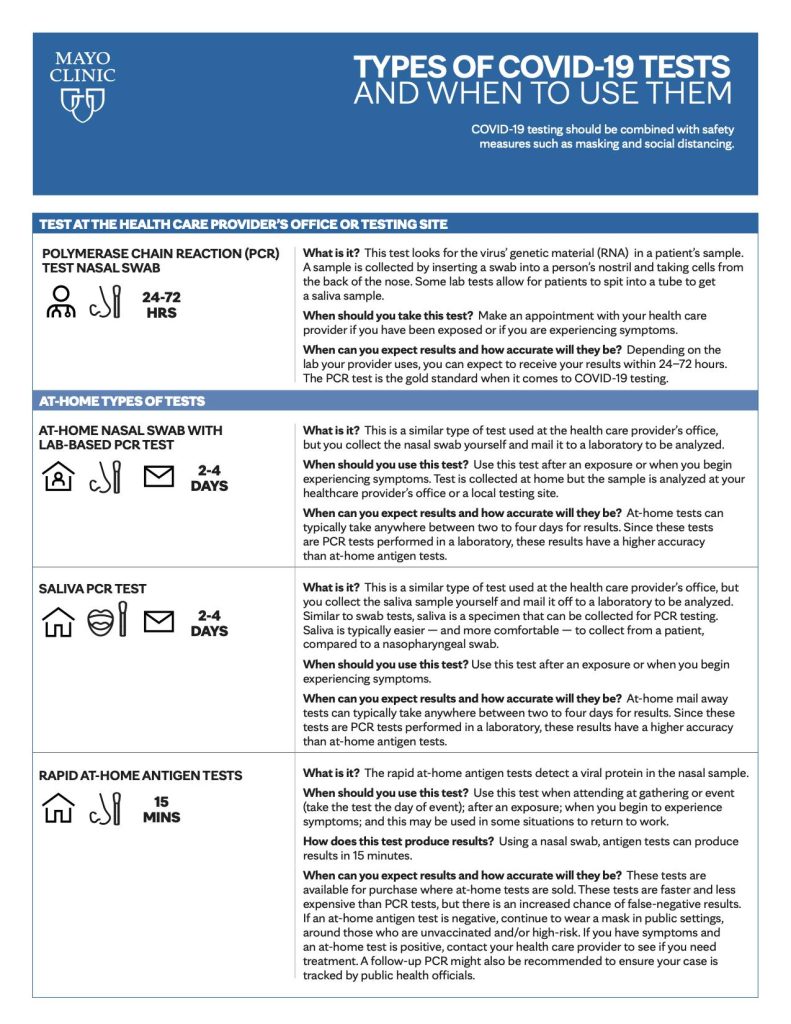
For a PDF version of the test chart.

Information in this post was accurate at the time of its posting. Due to the fluid nature of the COVID-19 pandemic, scientific understanding, along with guidelines and recommendations, may have changed since the original publication date . 

For more information and all your COVID-19 coverage, go to the  Mayo Clinic News Network  and  mayoclinic.org .

Learn more about  tracking COVID-19 and COVID-19 trends .

• Study finds that patients with alcohol-associated cirrhosis have worse outcomes in recovering from critical illness, compared with other cirrhosis patients Mayo Clinic Minute: Exercising in the new year

Related Articles

Understanding RT-PCR Tests and Results

• Published: 2021 March 16, 2021
• Author(s): Toby Le Aleksandra Wierzbowski
• Project No: 568
• PDF: Download PDF

Publication Summary

This document provides a brief description of the Real Time Reverse Transcriptase Polymerase Chain Reaction (RT-PCR) test. It provides basic information on how this molecular biology test is used in laboratories to detect genetic material of a pathogen such as SARS-CO-2 virus, the cause of COVID-19 disease.

COVID-19 Real-Time RT-PCR diagnostic tests can provide information on whether or not a patient has been infected with SARS-CoV-2 by detecting and measuring the virus’ genetic material.

This document provides a brief description of the Real Time Reverse Transcriptase Polymerase Chain Reaction (RT-PCR) test. It provides basic information on how this molecular biology test is used in laboratories to detect genetic material of a pathogen such as SARS-CO-2 virus, the cause of COVID-19 disease. It also provides the basics on interpreting test results that can be helpful in understanding the state of the disease and/or its progression and the likelihood of transmissibility. It can be of value to public health practitioners or anyone in healthcare community involved in the COVID-19 response.

What is a genetic material and how is it used to test for infectious diseases?

Genetic material is the instruction manual within a cell or virus that provides the directions on how to behave, survive and more. There are two types of genetic materials: Deoxyribonucleic acid (DNA) and Ribonucleic acid (RNA). The major difference between the two types of genetic materials is that DNA is a double-stranded structure whereas RNA is single-stranded. In terms of diagnostics, DNA is more stable for testing infectious disease than RNA because of its structural and intrinsic properties. It is also important to note that SARS-CoV-2 contains only RNA.

A common feature among all viruses is that they depend on host proteins and reproductive machinery for survival. Consequently, viruses like SARS-COV-2 are required to invade healthy cells in order to survive and multiply. Similar to other viruses, when SARS-COV-2 infiltrates a cell, it releases its RNA and exploits the cell’s machinery for viral replication. Furthermore, as long as the virus’ genetic material is present inside the cell, we can use a laboratory technique called Real-Time RT-PCR to determine whether a patient has been/is infected with SARS-CoV-2.

What is Real-Time RT-PCR?

Real-Time RT-PCR (Reverse Transcription Polymerase Chain Reaction) is a sensitive and fast test used for detecting the presence of specific genetic materials within a sample. This genetic material can be specific to humans, bacteria, and viruses like SARS-CoV-2.

The foundation of Real-Time RT-PCR derives from Polymerase Chain Reaction (PCR); a laboratory technique developed by Nobel Prize-winner, Kary B. Mullis, in the 1980s, to allow researchers to amplify and detect specific DNA targets (1,2). This technology was later improved to allow “real-time” visualization and quantification of DNA targets as they undergo amplification. To visualize the amplification of DNA, Real-time PCR uses increases in the fluorescence intensity of a fluorogenic probe in proportion to the amount of amplified DNA. By measuring this fluorescence intensity, one can quantify the amount of genetic material inside the sample. A major limitation of PCR is that it detects only DNA templates. Thus, in order to apply Real-Time PCR on RNA samples (i.e. genetic material of SARS-CoV-2), researchers have to use a special enzyme – called Reverse Transcriptase – to convert RNA into DNA templates, also known as complementary DNA (cDNA). Altogether, these features contribute to the versatility and sensitivity of Real-Time RT-PCR as a diagnostic test for infectious diseases.

How does Real-Time RT-PCR Work?

Sample Collection: To start the diagnostic test, a trained healthcare worker will use a swab to collect nasopharyngeal specimens from the patient’s nasopharynx. The sample is then placed into a sterile tube containing viral transport media to keep the virus viable (3).

Sample Preparation: Once the specimens arrive at the laboratory, researchers will use available commercial purification kits to extract RNA from the sample. Next, the RNA sample is added into one reaction mixture containing all the ingredients required to complete the diagnostic test, also known as “one-step RT-PCR”. The ingredients inside this mixture includes DNA polymerase, reverse transcriptase, DNA building blocks, and specific fluorophore probes and primers that recognize SARS-CoV-2.

Reverse Transcription: As mentioned earlier, PCR only works on DNA templates. Thus, the role of reverse transcriptase inside the reaction mixture is to convert all the RNA present within a given sample into cDNA. This includes human RNA, bacterial RNA, even other coronavirus RNA and if present, SARS-CoV-2’s RNA.

Step 1 – Denaturation/Separation: To begin, it is important to remember that DNA is a double-stranded structure. Thus, the next step is to unwind the DNA molecule into separate DNA stands. This is accomplished by heating the DNA to high temperatures (> 90°C) for amount 10 min.

Step 2 – Primer Annealing: Next, is the addition of short fragments of DNA, called primers. Primers are designed with high specificity and will attach to specific targets within cDNA of the SARS-CoV-2 RNA virus. The specific lower temperature is needed for primer annealing too. In general, there 7 common gene targets used for testing COVID-19; each gene target is essential to the virus’ replication or structure(4). Those essential gene targets include RNA-dependent polymerase (RdRP), ORF1ab (SARS-CoV-2’s conserved open reading frame), S gene (spike protein), N gene (nucleocapsid protein), E gene (envelope; virus’ outer shell).

Step 3 – Primer Extension/Elongation: Since DNA is a double stranded structure, there are two primers in this reaction mix, each one is designed to target one of the two DNA strands. Once the primers attach to their target DNAs, they will direct the DNA polyermase on where to begin and finish amplification on the DNA segment. This step results in an identical DNA copy of the target DNA.

And Repeat: Real-Time PCR will repeat the cycle multiple times (usually for 40 cycles). Every time RT-PCR completes a cycle, it will double the target DNA. Additionally, there are also fluorescent probes that bind specifically to the DNA targets, downstream of each primer. Every time DNA polyermase amplifies the DNA target, it will activate the probe to release a fluorescence signal. Thus, as the amount of target DNA increases, the fluorescence intensity will also increase.

What is the readout of Real-time RT-PCR?

The emitted fluorescence is then captured as a signal to generate a ‘cycle threshold’ (Ct) value. The Ct values refers to the amount of cycles required for the fluorescent signal to exceed background levels. Generally, the more target DNA that is in the sample, the faster its amplification will be and thus, the fewer cycles required before the fluorescence signal crosses the background threshold (lower Ct value). Conversely, if there are low amounts of target DNA, it will require more cycles before the fluorescence can cross the background threshold (higher Ct value).

Why are Ct values important?

Ct values are useful because they provide information about the patient’s pathogen genetic material load (SARS-CoV-2). A low Ct value indicates high viral genomic load, whereas a high Ct value indicates low viral genomic load. Health professionals can use Ct values in conjunction with clinical symptoms and history to gauge a patient’s stage of disease. Furthermore, serial Ct values generated from repeated testing can also help clinicians monitor the disease progression and predict stages of recovery and infection resolution. Contact tracers also utilizes Ct values to prioritize their attention to patients with the highest viral genomic load, which indicates a high risk for transmissibility.

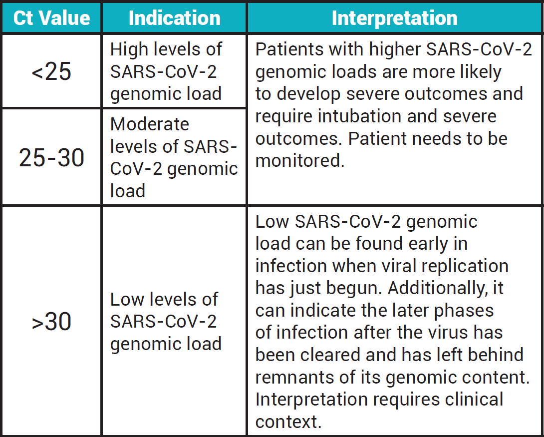
Select Your Interests

Customize your JAMA Network experience by selecting one or more topics from the list below.

• Academic Medicine
• Acid Base, Electrolytes, Fluids
• Allergy and Clinical Immunology
• American Indian or Alaska Natives
• Anesthesiology
• Anticoagulation
• Art and Images in Psychiatry
• Artificial Intelligence
• Assisted Reproduction
• Bleeding and Transfusion
• Caring for the Critically Ill Patient
• Challenges in Clinical Electrocardiography
• Climate and Health
• Climate Change
• Clinical Challenge
• Clinical Decision Support
• Clinical Implications of Basic Neuroscience
• Clinical Pharmacy and Pharmacology
• Complementary and Alternative Medicine
• Consensus Statements
• Coronavirus (COVID-19)
• Critical Care Medicine
• Cultural Competency
• Dental Medicine
• Dermatology
• Diabetes and Endocrinology
• Diagnostic Test Interpretation
• Drug Development
• Electronic Health Records
• Emergency Medicine
• End of Life, Hospice, Palliative Care
• Environmental Health
• Equity, Diversity, and Inclusion
• Facial Plastic Surgery
• Gastroenterology and Hepatology
• Genetics and Genomics
• Genomics and Precision Health
• Global Health
• Guide to Statistics and Methods
• Hair Disorders
• Health Care Delivery Models
• Health Care Economics, Insurance, Payment
• Health Care Quality
• Health Care Reform
• Health Care Safety
• Health Care Workforce
• Health Disparities
• Health Inequities
• Health Policy
• Health Systems Science
• History of Medicine
• Hypertension
• Images in Neurology
• Implementation Science
• Infectious Diseases
• Innovations in Health Care Delivery
• JAMA Infographic
• Law and Medicine
• Leading Change
• Less is More
• LGBTQIA Medicine
• Lifestyle Behaviors
• Medical Coding
• Medical Devices and Equipment
• Medical Education
• Medical Education and Training
• Medical Journals and Publishing
• Mobile Health and Telemedicine
• Narrative Medicine
• Neuroscience and Psychiatry
• Notable Notes
• Nutrition, Obesity, Exercise
• Obstetrics and Gynecology
• Occupational Health
• Ophthalmology
• Orthopedics
• Otolaryngology
• Pain Medicine
• Palliative Care
• Pathology and Laboratory Medicine
• Patient Care
• Patient Information
• Performance Improvement
• Performance Measures
• Perioperative Care and Consultation
• Pharmacoeconomics
• Pharmacoepidemiology
• Pharmacogenetics
• Pharmacy and Clinical Pharmacology
• Physical Medicine and Rehabilitation
• Physical Therapy
• Physician Leadership
• Population Health
• Primary Care
• Professional Well-being
• Professionalism
• Psychiatry and Behavioral Health
• Public Health
• Pulmonary Medicine
• Regulatory Agencies
• Reproductive Health
• Research, Methods, Statistics
• Resuscitation
• Rheumatology
• Risk Management
• Scientific Discovery and the Future of Medicine
• Shared Decision Making and Communication
• Sleep Medicine
• Sports Medicine
• Stem Cell Transplantation
• Substance Use and Addiction Medicine
• Surgical Innovation
• Surgical Pearls
• Teachable Moment
• Technology and Finance
• The Art of JAMA
• The Arts and Medicine
• The Rational Clinical Examination
• Tobacco and e-Cigarettes
• Translational Medicine
• Trauma and Injury
• Treatment Adherence
• Ultrasonography
• Users' Guide to the Medical Literature
• Vaccination
• Venous Thromboembolism
• Veterans Health
• Women's Health
• Workflow and Process
• Wound Care, Infection, Healing
• Download PDF
• Share X Facebook Email LinkedIn
• Permissions

Interpreting Diagnostic Tests for SARS-CoV-2

• 1 Department of Microbiology, Apollo Hospitals, Chennai, India
• 2 Department of Microbiology, Yokohama City University, Yokohama, Japan
• Research Letter RT-PCR Test Results in Patients Recovered From COVID-19 Lan Lan, MD; Dan Xu, MD; Guangming Ye, MD; Chen Xia, MS; Shaokang Wang, MS; Yirong Li, MD, PhD; Haibo Xu, MD, PhD JAMA
• Viewpoint Diagnostic Testing for the Novel Coronavirus Joshua M. Sharfstein, MD; Scott J. Becker, MS; Michelle M. Mello, JD, PhD JAMA
• Research Letter Antibodies in Infants Born to Mothers With COVID-19 Hui Zeng, MD; Chen Xu, BS; Junli Fan, MD; Yueting Tang, PhD; Qiaoling Deng, MD; Wei Zhang, MD, PhD; Xinghua Long, MD, PhD JAMA
• JAMA Patient Page Testing Individuals for COVID-19 Joseph Hadaya, MD; Max Schumm, MD; Edward H. Livingston, MD JAMA
• Medical News & Perspectives Could Frequent Testing Help Squelch COVID-19? Rita Rubin, MA JAMA

The pandemic of coronavirus disease 2019 (COVID-19) continues to affect much of the world. Knowledge of diagnostic tests for severe acute respiratory syndrome coronavirus 2 (SARS-CoV-2) is still evolving, and a clear understanding of the nature of the tests and interpretation of their findings is important. This Viewpoint describes how to interpret 2 types of diagnostic tests commonly in use for SARS-CoV-2 infections—reverse transcriptase–polymerase chain reaction (RT-PCR) and IgM and IgG enzyme-linked immunosorbent assay (ELISA)—and how the results may vary over time ( Figure ).

Estimated time intervals and rates of viral detection are based on data from several published reports. Because of variability in values among studies, estimated time intervals should be considered approximations and the probability of detection of SARS-CoV-2 infection is presented qualitatively. SARS-CoV-2 indicates severe acute respiratory syndrome coronavirus 2; PCR, polymerase chain reaction.

a Detection only occurs if patients are followed up proactively from the time of exposure.

b More likely to register a negative than a positive result by PCR of a nasopharyngeal swab.

Detection of Viral RNA by RT-PCR

Thus far, the most commonly used and reliable test for diagnosis of COVID-19 has been the RT-PCR test performed using nasopharyngeal swabs or other upper respiratory tract specimens, including throat swab or, more recently, saliva. A variety of RNA gene targets are used by different manufacturers, with most tests targeting 1 or more of the envelope ( env ), nucleocapsid ( N ), spike ( S ), RNA-dependent RNA polymerase ( RdRp ), and ORF1 genes. The sensitivities of the tests to individual genes are comparable according to comparison studies except the RdRp-SARSr (Charité) primer probe, which has a slightly lower sensitivity likely due to a mismatch in the reverse primer. 1

In most individuals with symptomatic COVID-19 infection, viral RNA in the nasopharyngeal swab as measured by the cycle threshold (Ct) becomes detectable as early as day 1 of symptoms and peaks within the first week of symptom onset. The Ct is the number of replication cycles required to produce a fluorescent signal, with lower Ct values representing higher viral RNA loads. A Ct value less than 40 is clinically reported as PCR positive. This positivity starts to decline by week 3 and subsequently becomes undetectable. However, the Ct values obtained in severely ill hospitalized patients are lower than the Ct values of mild cases, and PCR positivity may persist beyond 3 weeks after illness onset when most mild cases will yield a negative result. 2 However, a “positive” PCR result reflects only the detection of viral RNA and does not necessarily indicate presence of viable virus. 3

In some cases, viral RNA has been detected by RT-PCR even beyond week 6 following the first positive test. A few cases have also been reported positive after 2 consecutive negative PCR tests performed 24 hours apart. It is unclear if this is a testing error, reinfection, or reactivation. In a study of 9 patients, attempts to isolate the virus in culture were not successful beyond day 8 of illness onset, which correlates with the decline of infectivity beyond the first week. 3 That is in part why the “symptom-based strategy” of the Centers for Disease Control and Prevention (CDC) indicates that health care workers can return to work, if “at least 3 days (72 hours) have passed since recovery defined as resolution of fever without the use of fever-reducing medications and improvement in respiratory symptoms (e.g., cough, shortness of breath); and, at least 10 days have passed since symptoms first appeared.” 4

The timeline of PCR positivity is different in specimens other than nasopharyngeal swab. PCR positivity declines more slowly in sputum and may still be positive after nasopharyngeal swabs are negative. 3 In one study, PCR positivity in stool was observed in 55 of 96 (57%) infected patients and remained positive in stool beyond nasopharyngeal swab by a median of 4 to 11 days, but was unrelated to clinical severity. 2 Persistence of PCR in sputum and stool was found to be similar as assessed by Wölfel et al. 3

In a study of 205 patients with confirmed COVID-19 infection, RT-PCR positivity was highest in bronchoalveolar lavage specimens (93%), followed by sputum (72%), nasal swab (63%), and pharyngeal swab (32%). 5 False-negative results mainly occurred due to inappropriate timing of sample collection in relation to illness onset and deficiency in sampling technique, especially of nasopharyngeal swabs. Specificity of most of the RT-PCR tests is 100% because the primer design is specific to the genome sequence of SARS-CoV-2. Occasional false-positive results may occur due to technical errors and reagent contamination.

Detection of Antibodies to SARS-CoV-2

COVID-19 infection can also be detected indirectly by measuring the host immune response to SARS-CoV-2 infection. Serological diagnosis is especially important for patients with mild to moderate illness who may present late, beyond the first 2 weeks of illness onset. Serological diagnosis also is becoming an important tool to understand the extent of COVID-19 in the community and to identify individuals who are immune and potentially “protected” from becoming infected.

The most sensitive and earliest serological marker is total antibodies, levels of which begin to increase from the second week of symptom onset. 6 Although IgM and IgG ELISA have been found to be positive even as early as the fourth day after symptom onset, higher levels occur in the second and third week of illness.

For example, IgM and IgG seroconversion occurred in all patients between the third and fourth week of clinical illness onset as measured in 23 patients by To et al 7 and 85 patients by Xiang et al. 8 Thereafter IgM begins to decline and reaches lower levels by week 5 and almost disappears by week 7, whereas IgG persists beyond 7 weeks. 9 In a study of 140 patients, combined sensitivity of PCR and IgM ELISA directed at nucleocapsid (NC) antigen was 98.6% vs 51.9% with a single PCR test. During the first 5.5 days, quantitative PCR had a higher positivity rate than IgM, whereas IgM ELISA had a higher positivity rate after day 5.5 of illness. 10

ELISA-based IgM and IgG antibody tests have greater than 95% specificity for diagnosis of COVID-19. Testing of paired serum samples with the initial PCR and the second 2 weeks later can further increase diagnostic accuracy. Typically, the majority of antibodies are produced against the most abundant protein of the virus, which is the NC. Therefore, tests that detect antibodies to NC would be the most sensitive. However, the receptor-binding domain of S (RBD-S) protein is the host attachment protein, and antibodies to RBD-S would be more specific and are expected to be neutralizing. Therefore, using one or both antigens for detecting IgG and IgM would result in high sensitivity. 7 Antibodies may, however, have cross-reactivity with SARS-CoV and possibly other coronaviruses.

Rapid point-of-care tests for detection of antibodies have been widely developed and marketed and are of variable quality. Many manufacturers do not reveal the nature of antigens used. These tests are purely qualitative in nature and can only indicate the presence or absence of SARS-CoV-2 antibodies. The presence of neutralizing antibodies can only be confirmed by a plaque reduction neutralization test. However, high titers of IgG antibodies detected by ELISA have been shown to positively correlate with neutralizing antibodies. 7 The long-term persistence and duration of protection conferred by the neutralizing antibodies remains unknown.

Conclusions

Using available evidence, a clinically useful timeline of diagnostic markers for detection of COVID-19 has been devised ( Figure ). Most of the available data are for adult populations who are not immunocompromised. The time course of PCR positivity and seroconversion may vary in children and other groups, including the large population of asymptomatic individuals who go undiagnosed without active surveillance. Many questions remain, particularly how long potential immunity lasts in individuals, both asymptomatic and symptomatic, who are infected with SARS-CoV-2.

Corresponding Author: Sundararaj Stanleyraj Jeremiah, MD, Department of Microbiology and Molecular Biodefense Research, Yokohama City University School of Medicine, 3-9 Fukuura, Kanazawa-ku, Yokohama 236-0004, Japan ( [email protected] ).

Published Online: May 6, 2020. doi:10.1001/jama.2020.8259

Conflict of Interest Disclosures: None reported.

See More About

Sethuraman N , Jeremiah SS , Ryo A. Interpreting Diagnostic Tests for SARS-CoV-2. JAMA. 2020;323(22):2249–2251. doi:10.1001/jama.2020.8259

Manage citations:

© 2024

Artificial Intelligence Resource Center

Cardiology in JAMA : Read the Latest

Browse and subscribe to JAMA Network podcasts!

Others Also Liked

• Register for email alerts with links to free full-text articles
• Access PDFs of free articles
• Manage your interests
• Save searches and receive search alerts

• Skip to Main Content
• ePortfolios Directory

Igor Popovich

• Portfolio training 1
• Portfolio training 2
• Portfolio training 3
• Pre-lab 1. Fundamental Lab Skills
• Pre-lab 2. PCR Lab
• Pre-lab 3. Mitotic Index
• Lab report 1. Fundamental Lab Skills - Serial Dilution, Dilutions and Solution Prep

Lab report 2. PCR Lab

• Pre-lab 4. Corn Genetics
• Pre-lab 5. Southern Blot Analysis - Sickle Cell Diagnosis Lab
• Lab report 3. Mitotic Index
• Lab report 4. Corn Genetics
• Yeast pre-lab: Week 1
• Lab report 5. Letter to the child’s parents to report the results
• Yeast pre-lab: Week 2
• Lab report 6. From Genes to Proteins to Behavior Project

Name: Igor Popovich

Lab partner: Lada Grigorieva

Professor: Paul Kasili, Ph.D.

Class: BIO 208-01

Date: 1 February 2016

Abstract: Polymerase Chain Reaction (PCR) technique is a crucial procedure in molecular biology, which is used to amplify needed sequences of DNA and to generate thousands to millions of a particular DNA sequence. Our major purpose of this experiment is to learn how to perform PCR technique in order to avoid errors in further laboratory works. To perform the experiment, we obtained DNA template, primers, distilled water, and BIOMIX to combine them in tubes in a right volume according to the table in a manual. Having performed the procedure to prepare PCR products for a further usage in electrophoresis, we loaded PCR products into agarose gel and run gel at 120V. The results showed that the experiment was correctly done because each amplified DNA was separated properly according to the knowledge of how many base pairs each primer produces. Also, the result showed the same “picture” with the expected results in a manual. The PCR products from the tubes number 1 and 4 traveled the greatest distance because the combination of primers 1 and 2 in the first tube and the combination of primers 1,2, and 3 in the fourth tube produced approximately 550 base pairs. The PCR product from the tube number 2 traveled less distance, as the combination of primers 1 and 3 gave around 1025 base pairs. Finally, the PCR product from the tube number 3 almost did not travel because primer 1 generated small amounts of DNA. Thus, we have learned the proper usage of PCR technique and observed how different primers as well as their combinations amplify DNA, affecting the length.

Introduction: PCR (Polymerase Chain Reaction) is a procedure that is used to amplify a DNA sequence in order to generate thousands to millions of a particular DNA sequence. This technique was developed by Kary Millis in 1983, which became a frequently used technique in biotechnology (“Polymerase Chain Reaction,” 2016). This technique frequently applies in researches, medicine, and forensic. Researches can study patterns of gene expression, where they can analyze, for example, tissues at their different stages to observe the activity of genes. In medicine, PCR technique is used to test DNA, whether it has genetic disease mutations; parents can be tested if they are carriers of diseases. In forensic laboratories technicians can perform PCR technique and to determine if two DNA samples at different crime scenes have the same sequence of nucleotides and belong to the same person (“Applications of PCR,” 2015).

Actually, to perform PCR scientists need the following reactants: template DNA, Taq polymerase, is an enzyme, which adds nucleotides to a new strand of DNA, primers, appropriate buffer solution (provides a suitable environment for enzymes), and dNTPs , nucleotides that contain triphosphate groups (“Polymerase Chain Reaction,” 2016).

Basically, PCR technique consists of three steps: denaturation, annealing, and elongation. Each step should be properly performed to obtain needed results. Denaturation requires heating of original DNA at 95 Celsius degrees to separate double-stranded DNA into two strands. During the annealing, DNA is cooled to 45-72 Celsius degrees. Thus, primers can bind to the complementary sequences in the template DNA. When the elongation occurs, DNA polymerase starts to work extending primers. So, using DNA as a template, DNA polymerase adds nucleotides onto the primer, extending DNA strand in general (“PCR: How We Copy DNA.”).

Purpose:  The purpose of this experiment is to learn how to perform Polymerase Chain Reaction technique and to investigate how different primers as well as their combinations amplify DNA.

Hypothesis: If all steps for PCR technique were correctly done and the proper volume of reagents was added to each of the tubes, then we will obtain around 550 base pairs for the first and fourth tube, approximately 1025 base pairs for the second tube, and small amounts of DNA for the third tube. So, after gel electrophoresis, we will observe that the PCR products from the tubes number 1 and 4 will travel the greatest distance, the PCR product from the tube number 2 will travel less distance, and the PCR product from the tube number 3 will travel the smallest distance.

• DNA template: (conc. = 12.5 ng/μl)
• Primer 1 (12.5 μM)
• Primer 2 (12.5 μM)
• Primer 3 (12.5 μM)
• Distilled water
• BIOMIX – contains Taq DNA polymerase, dNTPs, Mg2+, and buffering salts
• Micropipettors (P 20, P 200)
• Picofuge tubes
• 1% agarose gel
• Electrophoresis apparatus

Procedure: Gloves were put on. The table was wiped down with a disinfectant. Picofuge tubes were obtained and labeled from 1 to 4. The reagents, which are shown in the table in a manual, were added. After, 15 μl of mineral oil were added to each tube. The PCR tubes were placed into the preprogrammed PCR machine. On the next week, these 4 tubes were taken back. A rack was obtained as well as 8 microfuge tubes (two microfuge tubes for each picofuge tube). 20 μl of PCR product were transferred from picofuge tube 1 and pipetted into microfuge tube 1A. Then, 10 μl were withdrawn from microfuge tube 1A and pipetted into new microfuge tube, 1B. So, each microfuge tube had 10 μl of PCR product. 5 μl of gel loading dye were added to tubes 1A and 1B. The procedure was repeated for picofuge 2,3, and 4. The tube contents were spun down in the microcentrifuge. After, the tubes were heated at 70 Celsius degrees for 3 minutes in a water bath. The agarose gel, buffer, and electrophoresis apparatus were obtained; the system was established. PCR products as well as DNA marker were loaded into a gel. Gel was run at 120V for 45 minutes. The bands were visualized using a UV box.     

Figure 1 shows the obtained results after gel electrophoresis. L-R: DNA ladder, tube 1A, tube 1B, tube 2A, tube 2B, tube 3A, tube 3B, tube 4A, and tube 4B.

Discussion: To learn PCR technique, we performed Polymerase Chain Reaction using 3 primers. The overall results showed that the procedure was properly done and the needed result was obtained.

According to the figure 1, our obtained gel electrophoresis is similar to the “expected results” picture in a manual. According to the knowledge of how many basic pairs each combination of primers can synthesize, we observed that the PCR product from the tube number 1, where we added the combination of primers 1 and 2, traveled the greatest distance (along with the PCR product from the fourth tube), as around 550 base pairs was synthesized; the smaller number of base pairs is synthesized, the greater distance it travels. However, if the amount of DNA was produced in an insufficient quantities or concentrations, as it was shown in the PCR product from the third tube (where we used only one primer, primer 1), PCR product cannot travel far away and we cannot observe an intense staining; the dye, which was added to the third tube, bound in insufficient quantities to the produced DNA. Talking about the PCR product from the second tube, the primer pair 1 and 3 gave approximately 1025 base pairs that allowed to the product to travel less distance; the greater number of base pairs is produced, the less distance it travels. Finally, the PCR product from the tube number 4 had approximately 550 base pairs (as it stopped on the same level with the PCR product number from tube 1), whereas we added combination of primers 1,2, and 3. So, why we could not also observe an intense staining at the same level with the PCR product from tube 2, where about 1025 bp were produced? The point is that the combination of primers 1,2 and 3 produces both, 550 bp and 1250 bp products, but randomly at each cycle. If 1025 bp product was produced from the template DNA, primer pair 1,2 can easily give a 550 bp product using this 1025 bp product. However, if 550 bp product was produced, primer pair 1, 3 cannot synthesize new 1025 bp product from this 550 bp product. Thus, after every cycle the amount of 550 bp products will be increased, whereas 1025 bp products will be reduced in quantity; so the dye will bind to small quantities of produced 1025 bp products and will not form an intense staining.

Conclusion:  Having performed the laboratory work, we learned the proper usage of PCR technique, where we performed the preparation of PCR products and run electrophoresis. The hypothesis was confirmed, and we observed that the PCR products from the tubes number 1 and 4 traveled the greatest distance, the PCR product from the tube number 2 traveled less distance, and the PCR product from the tube number 3 traveled the smallest distance. We learned that a loading dye having bound to very small amounts of produced DNA does not produce an intense staining, as was shown on the example of the PCR product from the tube 3. Also, when we combine primers to produce both, long strands (for example, 1025 bp) and short strands (550 bp) of DNA product, we will always have more of the shortest strands because long strands cannot be produced from the smaller one.

References:

“Applications of PCR.” Wikipedia, 11 September, 2015 ( https://en.wikipedia.org/wiki/Applications_of_PCR )

“PCR: How We Copy DNA.” Roche Molecular Diagnostics. ( http://molecular.roche.com/pcr/Pages/Process.aspx )

“Polymerase Chain Reaction.” Wikipedia, 5 February, 2016 ( https://en.wikipedia.org/wiki/Polymerase_chain_reaction )  

Work With Us- Join Our Team

Learn Genetics

How to Read, Interpret and Analyze Gel Electrophoresis Results?

Analyzing gel electrophoresis results and interpreting them, is a bit difficult task. One has to develop skills to read a gel. Let’s explore how you can do that with exclusively real gel examples. 

Gel electrophoresis is a conventional, native and subsidiary technique used to visualize DNA. There are two types of gel electrophoresis but we use conventional agarose gel electrophoresis so often. 

It requires an agarose polysaccharide that forms a porous structure for DNA to migrate. Using a colored marker the migration can be monitored and reported once the run is completed. 

Usually, Bromophenol blue is a dye used to track the migration, while EtBr is used to visualize DNA under UV light. The present technique is simple, handy and super useful, but still, requires a lot of experience. 

One has to have the expertise to perform, study, read and interpret the results. Often times students find it difficult to read gel results due to the lack of literature regarding this topic.

So I planned to write this article.

I have years of experience working in molecular laboratories. Using the best of my knowledge and expertise I will explain how you can read gel electrophoresis results. This article contains real gel images, some good and some bad. 

Actually, I especially collected such bad gel plates so that I can make you understand how good and bad things look in a gel. In the journey, first I will let you know how you can read the gel electrophoresis results. 

So this article would be a fun thing and a learning assignment for you and surely help you in your PCR and gel electrophoresis venture. 

Stay tuned. 

Key Topics:

How to read gel electrophoresis results? 

First, make clear if a gel contains any results or not. For that, put the gel carefully under the UV light and see if it contains any bands or not. 

In the second step, see if the gel possesses any visible contaminants like protein or RNA, or not. Contaminants have a direct effect on the purity of DNA and hence we have to identify them next.

If the gel has an RNA contaminant, the RNA bands will appear above the DNA. RNAs are smaller than DNA and thus migrate faster. So thick or many smear-like bands of RNA will appear above the DNA band which indicates RNA contamination. 

Likewise, if any thick band appears below the DNA, it will indicate protein contamination. The protein migrates behind the DNA in the gel. 

If any things mentioned here doesn’t appear in the gel, move ahead to investigate primer dimers. Primer dimer, in the case of PCR results, is an important marker that shows if the amplification occurred correctly or not. Here, some complementary nucleotides of both primers bind and amplify in the reaction.

Such products are short, usually 20 to 50 bp and appear at the bottom of the gel, far away from the DNA. If you see any faded band there, make sure you have primer dimers in the reaction. 

A thick band of genomic DNA, a linear and sharp band of PCR and a very sharp band of restriction digestion will appear in the gel. This is how you can read gel results. Take a look at the images below. 

Related article: Factor Affecting DNA Agarose Gel Electrophoresis Results .

Now take a look at some of the real gel pictures and discuss them one by one. 

Gel electrophoresis results of gDNA: 

This image is non-conclusive actually. But if you carefully observe well 9, the DNA is trying to come out from the gel. However, the smear indicates the contamination of RNA and DNA degradation. 

From 64 to 79, in each well DNA is trying to come out of the well but some DNA remained inside the well. A couple of reasons are responsible for that Firstly, the wells are broken during sample loading (see 72, 74, 75, 76, 77, 78) and secondly, the air bubbles were formed during the gel casting.

One another possibility in this gel is that the comb is not placed correctly or the gel is disturbed during the removal of the comb. Because of these reasons, the gDNA is unable to come out from the well.

Moreover, the smears above and below the DNA indicate contamination of RNA and protein. See wells 75, 76, 77, 78, 79. Conclusively, the DNA is not extracted properly and the gel preparation is poor.

This image is in two parts, part one, wells 48-55 is non-conclusive while part two from wells 56-63 shows some abnormalities. The best concentration of DNA is in the well 59, although due to poor gel preparation, it can’t come out properly. 

From wells 56 to 63, the gel wells are disrupted and also the DNA is contaminated with protein and RNA. 

Image 4 shows DNA degradation, contamination with RNA and proteins, poor gel preparations and unhealthy lab practices. Although, a substantially good amount of DNA is obtained in wells 45 and 47 but is of poor quality. 

Common problems in this gel are improper comb setup, poor gel quality, disrupted wells, etc. 

Now, this case is a bit different from other gels. Here the gel loading buffer is reused so many times, therefore, the actual concentration of the buffer is changed during the electrophoresis of this gel. Due to this reason,  the buffer limits the migration of DNA and therefore smears of DNA bands appeared.

Also, the gel is slightly brighter than other gels because of the presence of fragments of other previous DNA (in each run some amount of DNA remains in the buffer which appears in the next run when we re-use it).

This is a decent image of human blood genomic DNA extraction. You can see how intact the bands are and how beautiful it looks. This is an image of gDNA on 0.8% agarose gel. I also have added two other plates showing substantial RNA contamination in the gel. 

Related article: What is Electropherogram? How to Read it?

Gel electrophoresis results of PCR: 

The results of PCR are run on 2% gel with a clear and known DNA ladder. Now take a look at some of the results of PCR. 

The image is captured under the UV transilluminator instead of the gel doc system to show you the effect of EtBr on the gel electrophoresis results.

Here due to the re-use of a gel as well as the buffer, the EtBr is not properly spread into the gel. Further, the traces of the previous EtBr is also present in the gel. See the orange color near the wells, DNA and ladder. These all are the EtBr molecules not spread well.

Due to poor gel preparation, the ladder, as well as DNA, are not separated well. 

This image is very special, we have re-used gel and buffer many times. You can see the condition of DNA bands. Results are non-conclusive and fresh new electrophoresis gel and buffer are required here.  

Now this image is pretty good but what is the problem? You can see many bands, right? 

Here the annealing temperature of the primer is not selected properly. So the primer is compromised with other complementary sequences present in the genome. The annealing temperature is too low in comparison with its actual annealing temperature.

Due to this reason, more than 4 bands of PCR amplicons are observed in the gel. I also have noticed a minor thing. See the green arrow, it shows an air bubble in the gel. Conclusively, the PCR is not performed with the optimum PCR conditions.

Now this gel is pretty good, isn’t it? The DNA ladder is separated nicely and DNA is also appropriately amplified. But the concentration of the template DNA is a problem here.

The concentration of the template DNA used in this PCR reaction is very high. In a normal PCR reaction, 25 to 30ng concentration is sufficient. However, in this PCR reaction, the concentration of DNA will be more than 100ng.

The smear of the DNA along with the amplified product is observed due to this reason. And also two bands in some reactions, if you can see it. 

This gel is in very bad condition, nothing is good here. 

The shining dots in the gel are air bubbles. Due to the air bubbles, the ladder is not migrated properly see the first red arrow. Further, the ladder and DNA are too old, or not maintained properly, it’s degraded.

Now analyze this gel image, the DNA ladder ran faster than the samples. The samples are smeared as well which means that the buffer is too old, its concentration is altered or the pH of the buffer may be probably changed.

Remember, when we have the smears like this in any of the PCR products our buffer is the problem.

Now this image is pretty good but still has some problems. See the two red arrows, the bubbles which interfere with the migration of the DNA, and the higher concentration of the template DNA. 

We have seen all the types of DNA gel electrophoresis results and interpreted each type of electrophoresis results. But what qualities does a good-quality electrophoresis gel has?

• Good and sharp bands
• Minimum primer-dimers
• A beautifully separated DNA ladder.
• No background or traces of other DNA in the gel

See the next gel image and analyze each parameter. Though the primer dimers are present that is another issue. The result of the gel is beautiful and the bands are so clear and self-explanatory.

So after all these observations, I have a few suggestions which eventually help you more in this learning.

How to get good gel results? 

• Do not re-use the gel. If necessary use only twice.
• Do not reuse the buffer. If necessary use only twice or thrice.
• Prepare buffer freshly every time for the gel as well as the electrophoresis tank.
• Preserve DNA and DNA ladders properly in the cold chain.
• Use template DNA ~30ng to 50 ng not more than that, in the PCR reaction.
• Use only 10pMol primers. Follow PCR protocol.
• Use high-quality chemicals.

Read our next article in this series. The article is on the gel electrophoresis analysis of restriction digestion, cccDNA, linear DNA, supercoiled DNA and multiplex PCR: Part 2: Analysing and Interpreting (Agarose) Gel Electrophoresis Results .

Wrapping up: 

Getting good quality gel electrophoresis results is a matter of expertise. As you do it you will get mastery over time. Nonetheless, to sharpen your skills perform every step precisely.

Gel electrophoresis is an important genetic technique. It is used to validate the results of genomic DNA, PCR amplicons, restriction digestion and DNA library screening. I hope this article will help you in your genetics learning.  

Subscribe to our weekly newsletter for the latest blogs, articles and updates, and never miss the latest product or an exclusive offer.

Share this article

About The Author

Dr Tushar Chauhan

Related posts, chromosome- definition, structure, function and classification.

What is genome?- Definition, Structure and Function

25 thoughts on “How to Read, Interpret and Analyze Gel Electrophoresis Results?”

first of all thank you for this wonderful explanation. I want to ask a another question. what could be the reason of brightness in the UV absorbtion images?

Dna visualization uv rays cause disease so another technique use ????

No, we can only visualize DNA into UV with safety precautions.

My question is that in analysing and interpreting of the genomic DNA like in image 3 well 48,49,57 and 58?

We had loaded gDNA in those wells as well but it can’t be extracted or loaded correctly. That is why bands are not seen. We mean the whole gel is of gDNA samples. Some are contaminated, some are not migrated well, some are not extracted well etc. hope you understand.

Thank you it’s really helpfull

hello sir, your articles are so helpful and easy to understand. i am masters student and i always face problem in calculation part like if we are provided with this much of stock solution and have to make some amount of working from it. if you could please discuss about that it would be very kind of you.

Sure no prob. Give me tour email i will send you some material

[email protected] thankyou sir for your prompt response.

[email protected]

sir could you please also discuss about protein purification methods like SDS PAGE in future.

Hello Naidu. Our team is enthusiastic to write new things but unfortunately our blog niche is specific to DNA and Genetics so we cant discuss protein purification. But we will try to cover SDS PAGE.

good source of info

Thank You Ian Bremen

Very useful information

Very nice and helpful article. Thank you!!

thank you so much for appreciation

Hi, I had prepared a gel electrophoresis result for my dissertation. My lecturer had suggested that I comment about the level of expression of the mRNA. was wondering, what does she mean by this? How can we comment on level of expression of the mRNA?

Even i don’t understand your question? Can you reconferm your question?

Wow i really enjoy the content of this work.May God give you strength to do more.stay Blessed

Thank you so much Augustine

Thank you microbiology online notes. Appreciation from the giant platforms like you is a kind of achievement for us.

very nice content about electrophoresis easly understable keep doing like this..

WOW I REALLY ENJOY THE CONTENT OF THIS WORK IT’S WONDERFUL .MAY GOD GIVE YOU STRENGTH TO DO MORE.STAY BLESSED

Comments are closed.

Download our free PCR worksheet now. Available for a limited period. 

No thanks, I’m not interested!

Official websites use .gov

A .gov website belongs to an official government organization in the United States.

Secure .gov websites use HTTPS

A lock ( ) or https:// means you've safely connected to the .gov website. Share sensitive information only on official, secure websites.

SARS-CoV-2 Viral Shedding and Rapid Antigen Test Performance — Respiratory Virus Transmission Network, November 2022–May 2023

Weekly / April 25, 2024 / 73(16);365–371

Sarah E. Smith-Jeffcoat, MPH 1 ; Alexandra M. Mellis, PhD 2 ; Carlos G. Grijalva, MD 3 ; H. Keipp Talbot, MD 3 ; Jonathan Schmitz, MD, PhD 3 ; Karen Lutrick, PhD 4 ; Katherine D. Ellingson, PhD 4 ; Melissa S. Stockwell, MD 5 ,6 ,7 ; Son H. McLaren, MD 8 ; Huong Q. Nguyen, PhD 9 ; Suchitra Rao, MBBS 10 ; Edwin J. Asturias, MD 10 ; Meredith E. Davis-Gardner, PhD 11 ; Mehul S. Suthar, PhD 11 ; Hannah L. Kirking, MD 1 ; RVTN-Sentinel Study Group ( View author affiliations )

What is already known about this topic?

During the COVID-19 pandemic, rapid antigen tests were found to detect potentially transmissible SARS-CoV-2 infection, but antigen tests were less sensitive than reverse transcription–polymerase chain reaction (RT-PCR) testing.

What is added by this report?

During November 2022–May 2023, among persons infected with SARS-CoV-2, sensitivity of rapid antigen tests was 47% compared with RT-PCR and 80% compared with viral culture. Antigen tests continue to detect potentially transmissible infection but miss many infections identified by positive RT-PCR test results.

What are the implications for public health practice?

Rapid antigen tests can aid in identifying infectiousness of persons infected with SARS-CoV-2 and providing access to diagnostic testing for persons with COVID-19 symptoms. Persons in the community eligible for antiviral treatment should seek more sensitive diagnostic tests from a health care provider. Clinicians should consider RT-PCR testing for persons for whom antiviral treatment is recommended.

• Article PDF
• Full Issue PDF

As population immunity to SARS-CoV-2 evolves and new variants emerge, the role and accuracy of antigen tests remain active questions. To describe recent test performance, the detection of SARS-CoV-2 by antigen testing was compared with that by reverse transcription–polymerase chain reaction (RT-PCR) and viral culture testing during November 2022–May 2023. Participants who were enrolled in a household transmission study completed daily symptom diaries and collected two nasal swabs (tested for SARS-CoV-2 via RT-PCR, culture, and antigen tests) each day for 10 days after enrollment. Among participants with SARS-CoV-2 infection, the percentages of positive antigen, RT-PCR, and culture results were calculated each day from the onset of symptoms or, in asymptomatic persons, from the date of the first positive test result. Antigen test sensitivity was calculated using RT-PCR and viral culture as references. The peak percentage of positive antigen (59.0%) and RT-PCR (83.0%) results occurred 3 days after onset, and the peak percentage of positive culture results (52%) occurred 2 days after onset. The sensitivity of antigen tests was 47% (95% CI = 44%–50%) and 80% (95% CI = 76%–85%) using RT-PCR and culture, respectively, as references. Clinicians should be aware of the lower sensitivity of antigen testing compared with RT-PCR, which might lead to false-negative results. This finding has implications for timely initiation of SARS-CoV-2 antiviral treatment, when early diagnosis is essential; clinicians should consider RT-PCR for persons for whom antiviral treatment is recommended. Persons in the community who are at high risk for severe COVID-19 illness and eligible for antiviral treatment should seek testing from health care providers with the goal of obtaining a more sensitive diagnostic test than antigen tests (i.e., an RT-PCR test).

Introduction

SARS-CoV-2 rapid antigen tests were developed and received Food and Drug Administration Emergency Use Authorization early during the COVID-19 pandemic.* These tests were initially rolled out broadly in the United States to diagnose cases and isolate persons who received positive test results to aid in preventing onward spread at a time when population SARS-CoV-2 immunity was low, and rates of severe COVID-19–associated outcomes were high. In addition, demands for testing exceeded supply, and long turnaround times for reverse transcription–polymerase chain reaction (RT-PCR) test results contributed to ongoing transmission. Wide access to antigen tests was made possible through U.S. government initiatives implemented to prevent transmission. † , § After the emergence of the Omicron variant in late 2021, at-home antigen test use began to increase sharply ( 1 , 2 ).

Studies conducted during circulation of SARS-CoV-2 pre-Delta and Delta variants illustrated that antigen tests have high specificity, but lower sensitivity when compared with RT-PCR tests, thereby missing a substantial number of infections but correlating more closely with viral culture results ( 3 – 6 ). Viral culture, although not frequently used for routine patient care, is able to detect actively replicating virus (thus identifying when a person is likely to be infectious), whereas RT-PCR cannot distinguish between replicating virus and viral fragments. Most of these studies included few participants with vaccine- or infection-induced immunity. SARS-CoV-2 variants and population immunity have evolved since many of the studies assessing antigen tests were performed; thus, the role that antigen tests should play in diagnosing SARS-CoV-2 infection remains an active question. The objective of this investigation was to reevaluate the performance characteristics of SARS-CoV-2 antigen tests with those of RT-PCR and viral culture tests during a period with greater population immunity and more recently circulating SARS-CoV-2 Omicron variants.

This evaluation included participants enrolled in an antigen test substudy within a case-ascertained household transmission study during November 2022–May 2023 ¶ ( 7 ). Index patients with confirmed SARS-CoV-2 infection and their household contacts were enrolled within 7 days of illness onset in the index patient. Participants completed baseline surveys including demographic characteristics, COVID-19 signs or symptoms (symptoms),** vaccination, †† and self-reported previous infection. Participants (index patients and contacts) also provided a blood specimen for SARS-CoV-2 anti-N antibody detection §§ ( 8 , 9 ). For 10 days after enrollment, all participants completed daily COVID-19 symptom diaries and collected two nasal swabs each day. One swab was self-collected in viral transport media, stored in refrigerator for up to 72 hours, then collected by a study team member and stored at −12°F (−80°C) until aliquoted for automated RT-PCR (Hologic Panther Fusion) ¶¶ and viral culture,*** and the other swab was used for at-home antigen testing. ††† Participants interpreted and reported their antigen test results in their daily symptom diary. For this analysis, SARS-CoV-2 infection was defined as at least one positive RT-PCR test result during the study period; onset was defined as the first day of symptoms or, if the participant remained asymptomatic, day of first positive test result.

Among participants who ever received a positive RT-PCR test result and had one or more paired RT-PCR and antigen results reported, the percentage of positive antigen, RT-PCR, and viral culture results was calculated for each day relative to onset. The percentage of positive antigen test results was stratified by symptom and fever status. Sensitivity of antigen testing among paired samples collected from 2 days before until 10 days after onset was computed using two references: 1) same-day positive RT-PCR result and 2) same-day positive culture result, stratified by overall symptom status and presence of fever alone or fever or cough. Wilson score intervals were used for calculating 95% CIs around percentage of positive test results. Cluster-robust bootstrapping was used to calculate 95% CIs around sensitivity to account for within-participant correlation. All analyses were performed in RStudio (version 4.2.3; RStudio). This study was reviewed and approved by the Vanderbilt University Institutional Review Board. §§§

Characteristics of Study Participants

Among 354 participants in 129 households, 236 (67%) received a positive SARS-CoV-2 RT-PCR test result and were included in this investigation ( Table ). Participants ranged in age from 2 months to 83 years (median = 36 years; IQR = 17–50 years), 133 (56%) were non-Hispanic White persons, and 140 (59%) were female. Ninety-two (40%) participants reported receipt of a COVID-19 vaccine ≤12 months before enrollment; 82 (35%) had received ≥2 doses, but the most recent dose was >12 months before enrollment; 57 (24%) were unvaccinated (including those who had only ever received 1 dose); and vaccination status was unknown for five participants. A total of 102 (43%) participants had self-reported or serologic evidence of previous SARS-CoV-2 infection. At least one COVID-19 symptom was reported by 219 (93%) participants, including 182 (77%) who reported cough and 156 (66%) who reported fever.

SARS-CoV-2 Test Results

Among the 236 SARS-CoV-2–infected participants (i.e., those who received a positive RT-PCR test result), 2,244 antigen results were reported and included in analyses. Overall, 143 (61%) participants received one or more positive culture result, and 164 (69%) received one or more positive antigen test result.

The highest percentage of positive antigen (59%; 95% CI = 51%–67%) and RT-PCR (83%; 95% CI = 76%–88%) test results occurred 3 days after onset ( Figure 1 ). The highest percentage of positive viral culture results (52%; 95% CI = 43%–61%) occurred 2 days after onset. Among the 219 symptomatic participants, the highest percentage of positive antigen test results was 65% (95% CI = 57%–73%) at 3 days after onset among those who experienced any COVID-19 symptom and 80% (95% CI = 68%–88%) at 2 days after onset among those who reported fever.

Sensitivity of Antigen Testing

Compared with same-day collected RT-PCR and culture results, the overall sensitivities of daily antigen test results were 47% (95% CI = 44%–50%) and 80% (95% CI = 76%–85%), respectively ( Figure 2 ) (Supplementary Table, https://stacks.cdc.gov/view/cdc/153544 ). When stratified by symptoms experienced on the day of specimen collection, antigen test sensitivity increased with occurrence of any COVID-19 symptoms (56% and 85% compared with RT-PCR and culture, respectively) and peaked on days that fever was reported (77% and 94% compared with RT-PCR and culture, respectively). Compared with RT-PCR and culture results, sensitivity of antigen testing was low on days when no symptoms were reported (18% and 45%, respectively).

Among participants enrolled in a household transmission study during a period of increased disease- and vaccine-induced immunity, and when circulating viruses differed antigenically from the ancestral SARS-CoV-2 strain, antigen and culture tests detected a similar proportion of SARS-CoV-2 infections, but detection by RT-PCR was higher than that by either antigen or culture. Similarly, paired antigen test sensitivity was low compared with RT-PCR (47%), but relatively high compared with culture (80%). The sensitivity of antigen testing was higher when symptoms were present on the test day and peaked on days when participants reported fever. Although viral culture is not an absolute marker of transmissibility, this pattern suggests that positive antigen test results could indicate transmissible virus; thus, antigen tests might aid persons with COVID-19 in determining when they are no longer infectious once symptoms begin to resolve.

The findings from this investigation remain similar to those reported in other studies throughout the COVID-19 pandemic ( 3 – 6 ). For example, considering the current study’s sensitivity results, an early 2021 study comparing antigen testing with RT-PCR and culture found similar antigen test sensitivity compared with culture (84%), but slightly higher sensitivity compared with RT-PCR (64%) ( 3 ). The sensitivity difference between these two studies could be attributed to many factors, including differences in participant immunity, infecting variants, the limit of detection of the reference RT-PCR, or sampling methods.

Minimizing false negative test results is important because additional modalities, including antiviral medications, are available to prevent severe outcomes. Antiviral treatments for SARS-CoV-2 infection should be started as soon as possible, and within 5–7 days of symptom onset. ¶¶¶ Therefore, persons who are at higher risk for severe illness and eligible for antiviral treatment would benefit from a more accurate diagnostic test. In most clinical scenarios in the United States, this approach means a SARS-CoV-2 RT-PCR test would be a better diagnostic test to minimize the risk for a false-negative result. Alternatively, if RT-PCR tests are not available or accessible, clinicians and patients should follow FDA’s serial antigen testing recommendations to help optimize diagnostic test performance.****

Limitations

The findings in this report are subject to at least three limitations. First, participants included in this analysis might not represent all U.S. persons infected with SARS-CoV-2 and represent those with mild to moderate illness. These findings might not apply to persons with more severe COVID-19 illness. Second, one commercially available antigen test was used in this study; results might not apply to all available antigen tests. Finally, because of the parent study design, onset for asymptomatic participants (i.e., the day of the first positive test result), could be biased if household members were not enrolled early enough to record the earliest positive test result.

Implications for Public Health Practice

As COVID-19 becomes endemic and public focus shifts from stopping transmission to preventing severe illness, †††† diagnostic testing should emphasize use of the best tests to identify infection in persons who would benefit from treatment. The low sensitivity of antigen testing among persons with asymptomatic infections illustrates that these tests should only be used once symptoms are present. Conversely, the higher sensitivity when symptoms are present (especially cough or fever) supports the need to stay at home when symptomatic, irrespective of test result. §§§§ The low sensitivity of antigen tests compared with RT-PCR tests has implications for timely initiation of anti–SARS-CoV-2 treatment when early and accurate diagnosis is important. With several treatment options available, clinicians should consider more sensitive RT-PCR tests for accurate diagnosis in persons at higher risk for severe illness to minimize delays in treatment initiation. Persons in the community who are at high risk for severe COVID-19 illness and eligible for antiviral treatment should seek testing from health care providers with the goal of obtaining a more sensitive diagnostic test than antigen tests (i.e., an RT-PCR test).

Acknowledgments

Supraja Malladi, CDC; Erica Anderson, Marcia Blair, Jorge Celedonio, Daniel Chandler, Brittany Creasman, Ryan Dalforno, Kimberly Hart, Andrea Stafford Hintz, Judy King, Christopher Lindsell, Zhouwen Liu, Samuel Massion, Rendie E. McHenry, John Meghreblian, Lauren Milner, Catalina Padilla-Azain, Bryan Peterson, Suryakala Sarilla, Brianna Schibley-Laird, Laura Short, Ruby Swaim, Afan Swan, His-nien Tan, Timothy Williams, Paige Yates, Vanderbilt University Medical Center; Hannah Berger, Brianna Breu, Gina Burbey, Leila Deering, DeeAnn Hertel, Garrett Heuer, Sarah Kopitzke, Carrie Marcis, Jennifer Meece, Vicki Moon, Jennifer Moran, Miriah Rotar, Carla Rottscheit, Elisha Stefanski, Sandy Strey, Melissa Strupp, Murdoch Children’s Research Institute; Lisa Saiman, Celibell Y Vargas, Anny L. Diaz Perez, Ana Valdez de Romero, Raul A. Silverio Francisco, Columbia University.

RVTN-Sentinel Study Group

Melissa A. Rolfes, National Center for Immunization and Respiratory Diseases, CDC; Jessica E. Biddle, National Center for Immunization and Respiratory Diseases, CDC; Yuwei Zhu, Vanderbilt University Medical Center, Nashville, Tennessee; Karla Ledezma, University of Arizona, Tucson, Arizona; Kathleen Pryor, University of Arizona, Tucson, Arizona; Ellen Sano, Columbia University Irvin Medical Center, New York, New York; Joshua G. Petrie, Marshfield Clinic Research Institute, Marshfield, Wisconsin.

Corresponding author: Sarah E. Smith-Jeffcoat, [email protected] .

1 Coronavirus and Other Respiratory Viruses Division, National Center for Immunization and Respiratory Diseases, CDC; 2 Influenza Division, National Center for Immunization and Respiratory Diseases, CDC; 3 Vanderbilt University Medical Center, Nashville, Tennessee; 4 University of Arizona Colleges of Medicine and Public Health, Tucson, Arizona; 5 Division of Child and Adolescent Health, Department of Pediatrics, Vagelos College of Physicians and Surgeons, Columbia University, New York, New York; 6 Department of Population and Family Health, Mailman School of Public Health, New York, New York; 7 New York-Presbyterian Hospital, New York, New York; 8 Department of Emergency Medicine, Vagelos College of Physicians and Surgeons, Columbia University, New York, New York; 9 Marshfield Clinic Research Institute, Marshfield, Wisconsin; 10 Children’s Hospital Colorado, Aurora, Colorado; 11 Department of Pediatrics-Infectious Diseases, Emory Vaccine Center, Emory Primate Research Center, Emory University School of Medicine, Atlanta, Georgia.

All authors have completed and submitted the International Committee of Medical Journal Editors form for disclosure of potential conflicts of interest. Edwin J. Asturias reports grant support from Pfizer, consulting fees from Hillevax and Moderna, and payment from Merck for a lecture delivered at the Latin American Vaccine Summit. Carlos G. Grijalva reports support from the Food and Drug Administration and grants from the National Institutes of Health (NIH) and Syneos Health. Son H. McLaren reports institutional support from the Respiratory Virus Transmission Network, receipt of the Ken Graff Young Investigator Award from the American Academy of Pediatrics, Section on Emergency Medicine, institutional support from the National Center for Advancing Translational Science, the National Heart, Lung, and Blood Institute, and the Doris Duke Charitable Foundation COVID-19 Fund to Retain Clinician-Scientists. Suchitra Rao reports grant support from Biofire. Melissa S. Stockwell reports institutional support from the University of Washington, Boston Children’s Hospital, Westat, and New York University, and service as the Associate Director of the American Academy of Pediatrics Pediatric Research in Office Settings Research Network (payment to the trustees of Columbia University). Huong Q. Nguyen reports research support from CSL Seqirus, GSK, and ModernaTX, and an honorarium from ModernaTX for participating in a consultancy group, outside the submitted work. No other potential conflicts of interest were disclosed.

* https://www.fda.gov/news-events/press-announcements/coronavirus-covid-19-update-fda-authorizes-first-antigen-test-help-rapid-detection-virus-causes

† https://www.covid.gov/tools-and-resources/resources/tests

§ https://www.whitehouse.gov/wp-content/uploads/2021/01/National-Strategy-for-the-COVID-19-Response-and-Pandemic-Preparedness.pdf

¶ The Respiratory Virus Transmission Network sites that participated in the antigen substudy were located in Arizona, Colorado, New York, Tennessee, and Wisconsin. Persons who received test results positive for SARS-CoV-2 were recruited from participating medical centers, community testing sites, actively surveilled cohorts, and public health registries at five sites.

** Elicited COVID-19 symptoms included fever (including feeling feverish and chills), cough, sore throat, runny nose, nasal congestion, fatigue (including feeling run-down), wheezing, trouble breathing (including shortness of breath), chest tightness (including chest pain), loss of smell or loss of taste, headache, abdominal pain, diarrhea, vomiting, and muscle or body aches.

†† Vaccination history was self-reported and then verified by study team using state vaccination registries, electronic medical records, and pharmacy records.

§§ Detection of antinucleocapsid antibodies from a dried blood spot collected at baseline was considered serological evidence of previous SARS-CoV-2 infection. Simultaneous detection and differentiation of total binding antibody (immunoglobulin [Ig]M, IgG, and IgA) to SARS-CoV-2 2019-nCoV WHU02 strain nucleocapsid protein, Wuhan-Hu-1 strain spike protein receptor binding domain, and Wuhan-Hu-1 strain spike protein trimer in capillary (finger stick) dried blood was performed using the ProcartaPlex Immunoassay multiplex custom panel (Invitrogen) deployed on the MAGPIX System (Luminex).

¶¶ RT-PCR results were interpreted as categorically positive or negative according to the FDA-authorized parameters of the Hologic Panther Fusion SARS-CoV-2 assay, as utilized for in vitro diagnostic purposes. https://www.fda.gov/media/136156/download?attachment

*** Viral culture was performed on Vero E6 cells expressing both ACE2 and TMPRSS2. Cells were infected with serial dilutions of virus in Dulbecco’s Modified Eagle Medium (DMEM) containing ciprofloxacin, and cytopathic effect (CPE) was visually observed during a period of 5 days. Observation of CPE was considered positive for viral culture.

††† Quidel QuickVue At-Home COVID-19 Test (available as over-the-counter). https://www.fda.gov/media/146312/download

§§§ 45 C.F.R. part 46.114; 21 C.F.R. part 56.114.

¶¶¶ https://www.cdc.gov/coronavirus/2019-ncov/your-health/treatments-for-severe-illness.html

**** https://www.fda.gov/medical-devices/safety-communications/home-covid-19-antigen-tests-take-steps-reduce-your-risk-false-negative-results-fda-safety

†††† https://www.cdc.gov/respiratory-viruses/whats-new/changing-threat-covid-19.html

§§§§ https://www.cdc.gov/respiratory-viruses/prevention/precautions-when-sick.html

• Qasmieh SA, Robertson MM, Rane MS, et al. The importance of incorporating at-home testing into SARS-CoV-2 point prevalence estimates: findings from a US national cohort, February 2022. JMIR Public Health Surveill 2022;8:e38196. https://doi.org/10.2196/38196 PMID:36240020
• Rader B, Gertz A, Iuliano AD, et al. Use of at-home COVID-19 tests—United States, August 23, 2021–March 12, 2022. MMWR Morb Mortal Wkly Rep 2022;71:489–94. https://doi.org/10.15585/mmwr.mm7113e1 PMID:35358168
• Chu VT, Schwartz NG, Donnelly MAP, et al.; COVID-19 Household Transmission Team. Comparison of home antigen testing with RT-PCR and viral culture during the course of SARS-CoV-2 infection. JAMA Intern Med 2022;182:701–9. https://doi.org/10.1001/jamainternmed.2022.1827 PMID:35486394
• Tu Y-P, Green C, Hao L, et al. COVID-19 antigen results correlate with the quantity of replication-competent SARS-CoV-2 in a cross-sectional study of ambulatory adults during the Delta wave. Microbiol Spectr 2023;11:e0006423. https://doi.org/10.1128/spectrum.00064-23 PMID:37097146
• Almendares O, Prince-Guerra JL, Nolen LD, et al.; CDC COVID-19 Surge Diagnostic Testing Laboratory. Performance characteristics of the Abbott BinaxNOW SARS-CoV-2 antigen test in comparison to real-time reverse transcriptase PCR and viral culture in community testing sites during November 2020. J Clin Microbiol 2022;60:e0174221. https://doi.org/10.1128/JCM.01742-21 PMID:34705535
• Currie DW, Shah MM, Salvatore PP, et al.; CDC COVID-19 Response Epidemiology Field Studies Team. Relationship of SARS-CoV-2 antigen and reverse transcription PCR positivity for viral cultures. Emerg Infect Dis 2022;28:717–20. https://doi.org/10.3201/eid2803.211747 PMID:35202532
• Rolfes MA, Talbot HK, Morrissey KG, et al. Reduced risk of SARS-CoV-2 infection among household contacts with recent vaccination and previous COVID-19 infection: results from two multi-site case-ascertained household transmission studies. medRxiv [Preprint posted online October 21, 2023]. https://doi.org/10.1101/2023.10.20.23297317
• Chen L, Liu W, Zhang Q, et al. RNA based mNGS approach identifies a novel human coronavirus from two individual pneumonia cases in 2019 Wuhan outbreak. Emerg Microbes Infect 2020;9:313–9. https://doi.org/10.1080/22221751.2020.1725399 PMID:32020836
• Wu F, Zhao S, Yu B, et al. A new coronavirus associated with human respiratory disease in China. Nature 2020;579:265–9. https://doi.org/10.1038/s41586-020-2008-3 PMID:32015508

Abbreviations: RT-PCR = reverse transcription–polymerase chain reaction; SVI = Social Vulnerability Index. * SARS-CoV-2 infection defined as having received at least one positive RT-PCR result during study testing. † Persons of Hispanic or Latino (Hispanic) origin might be of any race but are categorized as Hispanic; all racial groups are non-Hispanic. § SVI was determined using the 2020 U.S. Census Bureau decennial tract location of the home. SVI uses 16 census variables to indicate the relative vulnerability of every census tract to a hazardous event with values closer to 1 representing highly vulnerable areas and values closer to 0 representing least vulnerable areas. ¶ Vaccination history was self-reported and then verified by study team. Participants were considered vaccinated within 12 months before enrollment if they had received ≥2 doses and the most recent dose was received between 14 days and 12 months before enrollment; vaccinated >12 months before enrollment if they had received ≥2 doses and the most recent dose was received >12 months before enrollment; and unvaccinated if they received <2 doses before enrollment. ** By self-report or serologic evidence. Previous SARS-CoV-2 infection was defined as self-report of a previous infection ≥1 month before enrollment or by detection of antinucleocapsid antibodies from a dried blood spot collected at baseline. †† Elicited COVID-19 signs and symptoms included fever (including feeling feverish or chills), cough, sore throat, runny nose, nasal congestion, fatigue (including feeling run-down), wheezing, trouble breathing (including shortness of breath), chest tightness (including chest pain), loss of smell or loss of taste, headache, abdominal pain, diarrhea, vomiting, and muscle or body aches.

FIGURE 1 . Percentage* of rapid antigen, reverse transcription–polymerase chain reaction, and viral culture test results that were positive for SARS-CoV-2 (A) and percentage of antigen test results that were positive, by symptom status† (B) and presence of fever (C) each day since onset § among participants infected with SARS-CoV-2 ¶ — Respiratory Virus Transmission Network, November 2022–May 2023

Abbreviation: RT-PCR = reverse transcription–polymerase chain reaction.

* With 95% CIs indicated by shaded areas.

† Elicited COVID-19 signs and symptoms included fever (including feeling feverish or chills), cough, sore throat, runny nose, nasal congestion, fatigue (including feeling run-down), wheezing, trouble breathing (including shortness of breath), chest tightness (including chest pain), loss of smell or loss of taste, headache, abdominal pain, diarrhea, vomiting, and muscle or body aches.

§ Date of symptom onset or, for asymptomatic persons, date of first positive test result.

¶ SARS-CoV-2 infection defined as having received at least one positive RT-PCR test result during study testing.

FIGURE 2 . Sensitivity* of rapid antigen tests results for diagnosing SARS-CoV-2 infection compared with reverse transcription–polymerase chain reaction (A) and viral culture (B), overall and by presence of symptoms † — Respiratory Virus Transmission Network, November 2022–May 2023

* With 95% CIs indicated by error bars.

Suggested citation for this article: Smith-Jeffcoat SE, Mellis AM, Grijalva CG, et al. SARS-CoV-2 Viral Shedding and Rapid Antigen Test Performance — Respiratory Virus Transmission Network, November 2022–May 2023. MMWR Morb Mortal Wkly Rep 2024;73:365–371. DOI: http://dx.doi.org/10.15585/mmwr.mm7316a2 .

MMWR and Morbidity and Mortality Weekly Report are service marks of the U.S. Department of Health and Human Services. Use of trade names and commercial sources is for identification only and does not imply endorsement by the U.S. Department of Health and Human Services. References to non-CDC sites on the Internet are provided as a service to MMWR readers and do not constitute or imply endorsement of these organizations or their programs by CDC or the U.S. Department of Health and Human Services. CDC is not responsible for the content of pages found at these sites. URL addresses listed in MMWR were current as of the date of publication.

All HTML versions of MMWR articles are generated from final proofs through an automated process. This conversion might result in character translation or format errors in the HTML version. Users are referred to the electronic PDF version ( https://www.cdc.gov/mmwr ) and/or the original MMWR paper copy for printable versions of official text, figures, and tables.

Exit Notification / Disclaimer Policy

• The Centers for Disease Control and Prevention (CDC) cannot attest to the accuracy of a non-federal website.
• Linking to a non-federal website does not constitute an endorsement by CDC or any of its employees of the sponsors or the information and products presented on the website.
• You will be subject to the destination website's privacy policy when you follow the link.
• CDC is not responsible for Section 508 compliance (accessibility) on other federal or private website.

Long-range and real-time PCR identification of a large SERPINC1 deletion in a patient with antithrombin deficiency

• Original Article
• Published: 27 May 2024

Cite this article

• Shinya Matsumoto   ORCID: orcid.org/0000-0001-5166-9036 1 ,
• Takeshi Uchiumi 2 , 3 ,
• Yasushi Ueyanagi 1 ,
• Nozomi Noda 1 ,
• Atsuhiko Sakai 4 ,
• Taeko Hotta 1 ,
• Kiyoko Kato 4 ,
• Shouichi Ohga 5 ,
• Yuya Kunisaki 1 , 2 &
• Dongchon Kang 1 , 6 , 7  

10 Accesses

Explore all metrics

Congenital antithrombin (AT) or serpin C1 deficiency, caused by a SERPINC1 abnormality, is a high-risk factor for venous thrombosis. SERPINC1 is prone to genetic rearrangement, because it contains numerous Alu elements. In this study, a Japanese patient who developed deep vein thrombosis during pregnancy and exhibited low AT activity underwent SERPINC1 gene analysis using routine methods: long-range polymerase chain reaction (PCR) and real-time PCR. Sequencing using long-range PCR products revealed no pathological variants in SERPINC1 exons or exon–intron junctions, and all the identified variants were homozygous, suggesting a deletion in one SERPINC1 allele. Copy number quantification for each SERPINC1 exon using real-time PCR revealed half the number of exon 1 and 2 copies compared with controls. Moreover, a deletion region was deduced by quantifying the 5′-upstream region copy number of SERPINC1 for each constant region. Direct long-range PCR sequencing with primers for the 5'-end of each presumed deletion region revealed a large Alu -mediated deletion (∼13 kb) involving SERPINC1 exons 1 and 2. Thus, a large deletion was identified in SERPINC1 using conventional PCR methods.

This is a preview of subscription content, log in via an institution to check access.

Access this article

Price includes VAT (Russian Federation)

Instant access to the full article PDF.

Rent this article via DeepDyve

Institutional subscriptions

Similar content being viewed by others

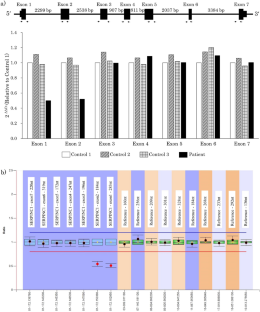
Identification and characterization of two SERPINC1 mutations causing congenital antithrombin deficiency

Testing for Factor V Leiden (FVL) and Prothrombin G20210A Genetic Variants

Genotyping of intron 22 inversion of factor viii gene for diagnosis of hemophilia a by inverse-shifting polymerase chain reaction and capillary electrophoresis, data availability.

The data that support the findings of this study are available from the corresponding author upon reasonable request.

Silverman GA, Bird PI, Carrell RW, Church FC, Coughlin PB, Gettins PC, et al. The serpins are an expanding superfamily of structurally similar but functionally diverse proteins. evolution, mechanism of inhibition, novel functions, and a revised nomenclature. J Biol Chem. 2001;276:33293–6.

Article   CAS   PubMed   Google Scholar  

Corral J, de la Morena-Barrio ME, Vicente V. The genetics of antithrombin. Thromb Res. 2018;169:23–9.

Tait RC, Walker ID, Perry DJ, Islam SI, Daly ME, McCall F, et al. Prevalence of antithrombin deficiency in the healthy population. Br J Haematol. 1994;87:106–12.

Pabinger I, Thaler J. How I treat patients with hereditary antithrombin deficiency. Blood. 2019;134:2346–53.

Article   PubMed   Google Scholar  

Ishiguro K, Kojima T, Kadomatsu K, Nakayama Y, Takagi A, Suzuki M, et al. Complete antithrombin deficiency in mice results in embryonic lethality. J Clin Invest. 2000;106:873–8.

Article   CAS   PubMed   PubMed Central   Google Scholar  

Bravo-Pérez C, de la Morena-Barrio B, Palomo A, Entrena L. Genotype-phenotype gradient of SERPINC1 variants in a single family reveals a severe compound antithrombin deficiency in a dead embryo. Br J Haematol. 2020;191:e32–5.

Corral J, Hernandez-Espinosa D, Soria JM, Gonzalez-Conejero R, Ordonez A, Gonzalez-Porras JR, et al. Antithrombin Cambridge II (A384S): an underestimated genetic risk factor for venous thrombosis. Blood. 2007;109:4258–63.

Tang LV, Tao Y, Feng Y, Ma J, Lin W, Zhang Y, et al. Gene editing of human iPSCs rescues thrombophilia in hereditary antithrombin deficiency in mice. Sci Transl Med. 2022;14:eabq3202.

Olds RJ, Lane DA, Chowdhury V, De Stefano V, Leone G, Thein SL. Complete nucleotide sequence of the antithrombin gene: evidence for homologous recombination causing thrombophilia. Biochemistry. 1993;32:4216–424.

Lee ST, Kim H-J, Kim D-K, Schuit RJ, Kim S-H. Detection of large deletion mutations in the SERPINC1 gene causing hereditary antithrombin deficiency by multiplex ligation-dependent probe amplification (MLPA). J Thromb Haemost. 2008;6:701–3.

Cordaux R, Batzer MA. The impact of retrotransposons on human genome evolution. Nat Rev Genet. 2009;10:691–703.

Ueki K, Nakamura K, Wakisaka Y, Wada S, Yoshikawa Y, Matsumot S, et al. An embolic stroke in a patient with PROC.p Lys193del. J Stroke Cerebrovasc Dis. 2020;29:104597.

Hamasaki N, Kuma H, Tsuda H. Activated protein C anticoagulant system dysfunction and thrombophilia in Asia. Ann Lab Med. 2013;33:8–13.

Yin T, Miyata T. Dysfunction of protein C anticoagulant system, main genetic risk factor for venous thromboembolism in Northeast Asians. J Thromb Thrombolysis. 2014;37:56–65.

Kimura R, Honda S, Kawasaki T, Tsuji H, Madoiwa S, Sakata Y, et al. Protein S-K196E mutation as a genetic risk factor for deep vein thrombosis in Japanese patients. Blood. 2006;107:1737–8.

Luxembourg B, Delev D, Geisen C, Geisen C, Spannagl M, Krause M, et al. Molecular basis of antithrombin deficiency. Thromb Haemost. 2011;105:635–46.

Tamura S, Hashimoto E, Suzuki N, Kakihara M, Odaira K, Hattori Y, et al. Molecular basis of SERPINC1 mutations in Japanese patients with antithrombin deficiency. Thromb Res. 2019;178:159–70.

Castaldo G, Cerbone AM, Guida A, Tandurella I, Ingino R, Tufano A, et al. Molecular analysis and genotype-phenotype correlation in patients with antithrombin deficiency from Southern Italy. Thromb Haemost. 2012;107:673–80.

García de Frutos P, Fuentes-Prior P, Hurtado B, Sala N. Molecular basis of protein S deficiency. Thromb Haemost. 2007;98:543–56.

Caspers M, Pavlova A, Driesen J, Harbrecht U, Klamroth R, Kadar J, et al. Deficiencies of antithrombin, protein C and protein S - practical experience in genetic analysis of a large patient cohort. Thromb Haemost. 2012;108:247–57.

De la Morena-Barrio B, Borràs N, Rodríguez-Alén A, de la Morena-Barrio ME, García-Hernández JL, Padilla J, et al. Identification of the first large intronic deletion responsible of type I antithrombin deficiency not detected by routine molecular diagnostic methods. Br J Haematol. 2019;186:e82–6.

PubMed   Google Scholar  

Cifuentes R, Padilla J, de la Morena-Barrio ME, de la Morena-Barrio B, Bravo-Pérez C, Garrido-Rodríguez P, et al. Usefulness and limitations of multiple ligation-dependent probe amplification in antithrombin deficiency. Int J Mol Sci. 2023;24:5023.

Kato I, Takagi Y, Ando Y, Nakamura Y, Murata M, Takagi A, et al. A complex genomic abnormality found in a patient with antithrombin deficiency and autoimmune disease-like symptoms. Int J Hematol. 2014;100:200–5.

Ma S, Zhang Z, Fu Y, Zhang M, Niu Y, Li R, et al. Identification of the first Alu-mediated gross deletion involving the BCKDHA gene in a compound heterozygous patient with maple syrup urine disease. Clin Chim Acta. 2021;517:23–30.

Pedini P, Laget L, Izard C, Menanteau C, Beley S, Granier T, et al. Identification of an Alu-mediated 5.7-kb deletion of the LU gene in a pregnant Moroccan woman with anti-Lu3. Blood Transfus. 2023;21:385–9.

PubMed   PubMed Central   Google Scholar  

Picard V, Chen JM, Tardy B, Aillaud M, Boiteux-Vergnes C, Dreyfus M, et al. Detection and characterisation of large SERPINC1 deletions in type I inherited antithrombin deficiency. Hum Genet. 2010;127:45–53.

Kibe T, Mori Y, Okanishi T, Shimojima K, Yokochi K, Yamamoto T. Two concurrent chromosomal aberrations involving interstitial deletion in 1q24.2q25.2 and inverted duplication and deletion in 10q26 in a patient with stroke associated with antithrombin deficiency and a patent foramen ovale. Am J Med Genet A. 2011;155A:215–20.

Gindele R, Selmeczi A, Oláh Z, Ilonczai P, Pfliegler G, Marján E, et al. Clinical and laboratory characteristics of antithrombin deficiencies: a large cohort study from a single diagnostic center. Thromb Res. 2017;160:119–28.

De la Morena-Barrio B, Stephens J, de la Morena-Barrio ME, Stefanucci L, Padilla J, Miñano A, et al. Long-read sequencing identifies the first retrotransposon insertion and resolves structural variants causing antithrombin deficiency. Thromb Haemost. 2022;122:1369–78.

Article   PubMed   PubMed Central   Google Scholar  

Download references

Acknowledgements

We would like to thank Editage ( www.editage.com ) for English language editing.

This work was supported in part by the Japan Society for the Promotion of Science (JSPS) KAKENHI [grant number: JP21K07319 to SM, JP23K18217 to TU and JP22H03537 to TU].

Author information

Authors and affiliations.

Department of Clinical Chemistry and Laboratory Medicine, Kyushu University Hospital, 3-1-1 Maidashi, Higashi-ku, Fukuoka, 812-8582, Japan

Shinya Matsumoto, Yasushi Ueyanagi, Nozomi Noda, Taeko Hotta, Yuya Kunisaki & Dongchon Kang

Department of Clinical Chemistry and Laboratory Medicine, Graduate School of Medical Sciences, Kyushu University, Fukuoka, Japan

Takeshi Uchiumi & Yuya Kunisaki

Department of Health Sciences, Graduate School of Medical Sciences, Kyushu University, Fukuoka, Japan

Takeshi Uchiumi

Department of Obstetrics and Gynecology, Graduate School of Medical Sciences, Kyushu University, Fukuoka, Japan

Atsuhiko Sakai & Kiyoko Kato

Department of Pediatrics, Graduate School of Medical Sciences, Kyushu University, Fukuoka, Japan

Shouichi Ohga

Kashiigaoka Rehabilitation Hospital, Fukuoka, Japan

Dongchon Kang

Department of Medical Laboratory Science, Faculty of Health Sciences, Junshin Gakuen University, Fukuoka, Japan

You can also search for this author in PubMed   Google Scholar

Corresponding author

Correspondence to Shinya Matsumoto .

Ethics declarations

Conflict of interest.

The authors declare that they have no conflict of interest.

Additional information

Publisher's note.

Springer Nature remains neutral with regard to jurisdictional claims in published maps and institutional affiliations.

Supplementary Information

Below is the link to the electronic supplementary material.

Supplementary file1 (DOCX 25 KB)

About this article.

Matsumoto, S., Uchiumi, T., Ueyanagi, Y. et al. Long-range and real-time PCR identification of a large SERPINC1 deletion in a patient with antithrombin deficiency. Int J Hematol (2024). https://doi.org/10.1007/s12185-024-03796-y

Download citation

Received : 25 January 2024

Revised : 10 May 2024

Accepted : 20 May 2024

Published : 27 May 2024

DOI : https://doi.org/10.1007/s12185-024-03796-y

Share this article

Anyone you share the following link with will be able to read this content:

Sorry, a shareable link is not currently available for this article.

Provided by the Springer Nature SharedIt content-sharing initiative

• Antithrombin deficiency
• Large deletion
• Long-range PCR
• Real-time PCR
• Find a journal
• Publish with us
• Track your research

• Open access
• Published: 24 May 2024

Effect of genomic and cellular environments on gene expression noise

• Clarice K. Y. Hong 1 , 2   na1 ,
• Avinash Ramu 1 , 2   na1 ,
• Siqi Zhao 1 , 2   na1 &
• Barak A. Cohen   ORCID: orcid.org/0000-0002-3350-2715 1 , 2  

Genome Biology volume  25 , Article number:  137 ( 2024 ) Cite this article

289 Accesses

Metrics details

Individual cells from isogenic populations often display large cell-to-cell differences in gene expression. This “noise” in expression derives from several sources, including the genomic and cellular environment in which a gene resides. Large-scale maps of genomic environments have revealed the effects of epigenetic modifications and transcription factor occupancy on mean expression levels, but leveraging such maps to explain expression noise will require new methods to assay how expression noise changes at locations across the genome.

To address this gap, we present Single-cell Analysis of Reporter Gene Expression Noise and Transcriptome (SARGENT), a method that simultaneously measures the noisiness of reporter genes integrated throughout the genome and the global mRNA profiles of individual reporter-gene-containing cells. Using SARGENT, we perform the first comprehensive genome-wide survey of how genomic locations impact gene expression noise. We find that the mean and noise of expression correlate with different histone modifications. We quantify the intrinsic and extrinsic components of reporter gene noise and, using the associated mRNA profiles, assign the extrinsic component to differences between the CD24+ “stem-like” substate and the more “differentiated” substate. SARGENT also reveals the effects of transgene integrations on endogenous gene expression, which will help guide the search for “safe-harbor” loci.

Conclusions

Taken together, we show that SARGENT is a powerful tool to measure both the mean and noise of gene expression at locations across the genome and that the data generatd by SARGENT reveals important insights into the regulation of gene expression noise genome-wide.

Gene expression is noisy, even among individual cells from an isogenic population [ 1 ]. Noisy gene expression leads to variable cellular outcomes in differentiation [ 2 , 3 , 4 , 5 ], the response to environmental stimuli [ 6 , 7 ], viral latency [ 8 ], and chemotherapeutic drug resistance [ 9 , 10 , 11 ]. Explaining the causes of noisy expression remains an important challenge.

A gene’s genomic environment, defined here as the composition of nearby cis -regulatory elements and local epigenetic marks, can influence its expression noise. Some features of genomic environments that can affect noise include enhancers, histone modifications, and transcription factor (TF) occupancy [ 12 , 13 , 14 , 15 , 16 , 17 , 18 ]. These observations raise the possibility that genome-wide patterns of expression noise could be explained using the large-scale epigenetic maps that have proved useful in explaining mean expression levels [ 19 , 20 , 21 ]. Leveraging these resources to explain expression noise will require maps of the genome that show the influence of diverse genomic environments on this noise. Producing these maps will require new experimental approaches because the existing studies demonstrating the effects of epigenetic marks on expression noise have either been performed on endogenous genes, where the effects of different chromosomal locations are confounded with the effects of the different endogenous promoters, or rely on low-throughput imaging methods. Dar et al. assayed the noisiness of large numbers of genomic integrations, but was unable to assign genomic locations to the measured reporter genes [ 15 ]. Two other studies have assayed integrations in a high-throughput manner but measured protein levels by flow cytometry rather than mRNA levels [ 22 , 23 ]. Even for the same reporter gene, noise in translational mechanisms can confound the measurements [ 24 ], especially when trying to understand the impact of features that regulate transcription. Thus, we still lack a high-throughput, systematic way of quantifying the impact of genomic environments on expression noise.

In addition to intrinsic features such as the local genomic environment, extrinsic features, such as the global cellular state of a cell, can also influence gene expression noise [ 25 , 26 , 27 , 28 , 29 ]. For example, variation in the cell cycle, cell size, or signaling pathways can all impact gene expression noise [ 1 , 30 , 31 ]. However, the relative contributions of intrinsic vs extrinsic features on gene expression noise in mammalian cells remains unclear.

Here we report Single-cell Analysis of Reporter Gene Expression Noise and Transcriptome (SARGENT), a highly parallel method to measure the mean and noise of a common reporter gene that has been integrated at locations across the genome. Analysis of SARGENT data showed that different histone modifications explain the mean and noise produced across the genome. In SARGENT, multiple reporters are integrated in each cell, allowing us to separate the intrinsic and extrinsic contributions to noise. A key advantage of SARGENT is that we can also sequence the associated single-cell mRNA transcriptomes, further enabling us to attribute the extrinsic noise to differences in the cellular substates between isogenic cells. To our knowledge, this is the largest genome-wide survey of the impact of intrinsic and extrinsic noise in gene expression. Taken together, our results show that SARGENT is a powerful tool to study how genomic environments and cellular context control expression noise.

A high-throughput method to measure mean and noise across the genome

We developed a high-throughput method to test the effects of genomic environments on the mean and noise of gene expression. Our goal was to integrate a common transgene across the genome and then, for individual cells, measure both the transcripts produced from the transgene and the global mRNA profile. This allows us to compute the mean and noise of reporter gene expression at each location and correlate reporter gene expression with the cellular mRNA state of each cell. Because every unique integration contains the same transgene, the measured differences in the mean and noise of reporter gene expression are directly attributable to the influence of genomic environments or cellular states.

We first generated a reporter gene with a library of 16 bp random barcodes (location barcode, locBC) in its 3’UTR (Fig. 1 ). Due to the diversity of the locBCs, each locBC is only associated with a single location in the genome [ 20 ]. The reporter gene consists of a cytomegalovirus (CMV) promoter driving the expression of a fluorescent protein and contains a capture sequence from the 10× Genomics Single Cell Gene Expression 3' v3.1 with Feature Barcoding Kit. We chose to use the CMV promoter because it is a general promoter that should respond to different enhancers and chromatin environments. The 10× gel beads contain both the complementary capture sequence and polyT sequences, allowing us to isolate the transcripts produced from the reporter gene and the cellular transcriptome.

Overview of the SARGENT workflow. In step 1, a reporter gene driven by the CMV promoter is randomly barcoded with a diverse library of location barcodes (locBC) upstream of the 10× capture sequence (CS). The reporter genes are randomly integrated into K562 cells and sorted for cells with successful integrations (step 2), then sorted again after a week into pools to ensure that each barcode is only represented once per pool (step 3). We then performed scRNA-seq to capture the transcriptome and amplify the expressed barcodes from integrated reporter genes (step 4). The number of expressed barcodes per cell were then tabulated (step 5). To identify the genomic locations of the integrations, we also mapped the location of each locBC with inverse PCR (step 6). ITR: inverted terminal repeat, prom: promoter

To generate chromosomal integrations across the genome, we cloned the reporter gene library onto a piggyBac transposon vector. We selected the piggyBac transposon system because it has a bias towards active chromatin regions where transcription is more likely to occur so that we are likely to detect the IRs by scRNA-seq. The library was transfected into cells along with piggyBac transposase to allow random integrations of the reporter into the genome. We performed SARGENT in K562 cells because of the abundance of public epigenetic data available for this cell line. After sorting the transfected cells for integrations, we mapped the locations of each integrated reporter (IR) and assigned each locBC to a specific genomic location. We then captured the reporter gene transcripts from single cells and amplified the barcodes (10× cell barcode, UMI, and locBC) using primers specific to our reporter gene (Fig. 1 , “  Methods ”). After sequencing and tabulating the mRNA counts for each IR, we computed the expression level of the reporter gene at each genomic location in each single cell. For a subset of cells, we also sequenced the mRNA profiles to simultaneously reveal the cell state of each individual cell.

SARGENT measurements are accurate and reproducible

We first assessed the reproducibility of the SARGENT method. Because replicate infections result in pools of cells with insertions at different genomic locations, we could not assess the reproducibility of independently transfected pools of cells. Instead, we assessed the reproducibility of SARGENT by growing the same pool of insertions (Pool 4) in separate flasks and performing the SARGENT workflow independently on each sample. We detected 589 identical IR locations in both replicates, which represented 96% of the total IRs observed in both replicates. After quality control, we obtained data from 7680 single cells across replicates, and a total of 2,940,912 unique molecular identifiers (UMIs) representing expressed barcodes from the IRs in these cells. The replicates were well correlated for measurements of both mean and noise measured at each IR location (Fig. 2 A, B, mean Pearson’s r = 0.76, noise Pearson’s r = 0.72) indicating that measurements obtained by SARGENT are reproducible. We combined the two technical replicates from Pool 4 for downstream analysis.

SARGENT measurements are accurate and reproducible. A Correlation of mean levels between technical replicates. B Correlation of variance measurements between replicates. C Mean and variance are correlated within each experiment. D Mean-independent noise corrects for mean effects on variance. Correlations shown are Pearson’s correlation coefficients (Pearson’s r )

To validate the single-cell measurements made by SARGENT, we also performed single-molecule fluorescence in situ hybridization (smFISH) on two known locations. At least for these two locations, the measurements of mean and variance made by smFISH qualitatively agree with the SARGENT measurements for those locations (Additional file 1 : Fig. S1) suggesting that our method is accurate and reproducible for measuring the mean and noise of expression.

Measurements of mean-independent noise across different chromosomal environments

In total, we performed four experiments and generated mean and noise measurements for 939 integrations (Additional file 2 : Table S1). The integrations were spread across the genome and found in regions with different chromHMM annotations [ 32 ] (Additional file 1 : Fig. S2A, S2B), allowing us to study the effects of diverse chromosomal environments on expression noise.The mean and variance of expression are often highly correlated [ 33 , 34 ]. Similarly, we found a strong correlation between the mean and variance in SARGENT data, indicating that a large proportion of an IR’s noise is explained by its mean level of expression (Fig. 2 C). To identify chromosomal features that control expression noise independent of mean levels we regressed out the effect of mean levels on noise, leaving us with a metric we refer to as mean-independent noise (MIN) [ 33 ]. By design, MIN levels of IRs are uncorrelated with their mean expression levels (Fig. 2 D) whereas other measures of noise, such as the coefficient of variation or the Fano factor, retain residual correlation with mean levels in our data (Additional file 1 : Fig. S2C, S2D). Thus, we used MIN as a measure of expression noise for all following analyses.

Expression mean and noise are associated with different chromosomal features

We sought to identify chromatin features that would explain differences in MIN levels between genomic locations. Studies of genome-wide chromatin features in many cell lines and tissues have shown that the mean expression of a gene is correlated with its surrounding chromatin marks [ 20 , 35 ]. Thus, we asked whether chromatin features might also explain patterns of MIN across the genome. We split the IRs into bins of high or low mean levels, or high or low MIN levels, and identified chromatin features that were correlated with each bin. As expected, IRs with high mean expression had higher levels of active chromatin marks such as H3K27ac, H3K4 methylation, H3K79me2, and H3K9ac (Fig. 3 A). Conversely, IRs with high MIN did not exhibit differences between H3K27ac or H3K4me1 levels, and low MIN locations showed slightly elevated levels of H3K4me2/3, H3K79me2, and H3K9ac (Fig. 3 B). To ensure that these results are not due to the presence of outlier IR locations, we also plotted the mean levels of each chromatin mark for each IR and showed that there are no individual IR locations that appear to be skewing the distribution (Additional file 1 : Fig. S3A, S3B). We also randomly permuted the mean/MIN labels to determine the significance of the differences we observed. For high/low mean levels, the differences observed for all chromatin modifications are significant, while for MIN levels, only H3K4me2/3 and H3K9ac are significant (Additional file 1 : Fig. S3C), suggesting that the differences observed above are robust. These results suggest that different chromatin modifications influence the mean and noisiness of expression and that more active genomic locations might also reduce MIN. This observation is consistent with previous studies showing that repressed chromatin is associated with high MIN [ 18 , 22 ].

Expression mean and noise are associated with different chromosomal features. A Active histone modifications associated with high or low mean IRs. Start indicates the location of the IR, and each location was extended 5 kb on either side. IRs that map to the minus strand were reverse complemented so the orientation with respect to the IR is consistent. B Active histone modifications associated with high or low MIN IRs are different from those associated with mean. C Motifs enriched in high or low MIN IRs respectively (STREME [ 36 ] P -value < 0.05), and potential TFs that match these discovered motifs. D Logistic regression weights of various intrinsic features associated with high or low MIN IRs. Red bars: p -value < 0.05; pink bars: 0.05 < p -value < 0.1 from the logistic regression model

The binding of TFs also impacts noise in gene expression. To identify TFs that might affect noise, we identified motifs whose occupancy is enriched near either high or low MIN IRs. Sequences at low MIN IRs are enriched for motifs that are bound by transcriptional activators such as SP1 and E2F4, while sequences at high MIN IRs are enriched for motifs that are bound by other TFs including TFs containing basic helix-loop-helix (bHLH) domains (Fig. 3 C), suggesting that the cofactors recruited by different TFs have separable effects on expression mean and noise. To further understand whether the identified motifs are functioning across multiple regions or are only enriched in a few regions, we plotted the distribution of occurrences of each motif in each region. Depending on the motif, each motif can occur ~0–5 times. Motifs enriched in high MIN regions occur in more high MIN regions and at slightly higher frequency in high MIN regions, while low MIN motifs are present in more low MIN regions (Additional file 1 : Fig. S3D, 3E). These results suggest that the TFs binding to these motifs act across many high/low MIN regions to modulate gene expression noise.

To assess the power of genomic features to predict the MIN of IR locations, we trained a logistic regression model using various chromatin modifications, sequence features, and genomic annotations to classify high and low MIN locations (total 37 features, full list of features in Additional file 3 : Table S2). The model achieved 59% accuracy using leave-one-out cross-validation (LOOCV). The features with significant weights are the H3K4me3 mark, TF motifs (RARG, FOXO4, HIF1A, TFAP4, CREM, ATF1, NFIC, and NFIA), and whether the IR location was inside a gene (Fig. 3 D, Additional file 3 : Table S2). Being inside a gene reduced the probability of being a high noise lR location, which could be due to local regulatory elements that might dampen gene expression noise for robust expression. Similar to our results above, lower H3K4me3 increased the probability of being a high noise IR location. H3K4me3 is associated with active chromatin and supports the hypothesis that higher activity reduces IR MIN. Our observation is consistent with a previous study showing that H3K4me3 correlates with reduced noise at endogenous genes [ 18 ]. With respect to the effects of TFs on noise, the presence of some TF motifs increases the probability of being a high noise IR location (NFIC, CREM, TFAP4, CLOCK), whereas other TFs reduce the probability of being a high noise location (RARG, NFIA, ATF1, FOXO4, HIF1A).

We used a similar logistic regression framework to identify features that separate IR locations with high or low mean levels of expression. The model accuracy is 66% using LOOCV. The chromatin features that increase the probability of being a high mean IR location are lower levels of H3K27me3, lower levels of H3K4me2, and a higher number of ATAC-seq peaks, which agrees with the known effects of these features in bulk mean expression. The motifs that increased the probability of being a high mean IR location are higher numbers of motifs of the ZNF76, BACH1, and E2F3 TFs and fewer instances of the E2F7, SMAD3, and SOX5 motifs. (Additional file 1 : Fig. S3F, Additional file 4 : Table S3). Comparisons of the models explaining either mean or noise again show that different genomic features are correlated with gene expression mean and noise.

Intrinsic and extrinsic factors have similar effects on gene expression noise

Expression noise caused by fluctuations in global factors affects all genes and is referred to as extrinsic noise, whereas intrinsic sources of noise are specific to individual genes [ 22 , 28 , 29 , 30 , 31 , 33 ]. The correlation between identical reporter genes in the same cell measures the balance between extrinsic and intrinsic noise, with extrinsic factors increasing the correlation [ 25 ]. In SARGENT, the correlation between IRs in the same cells is a measure of extrinsic factors that affect noise across IR locations.

For our analysis of extrinsic noise, we first identified IRs in the same clonal cells using the co-occurrence of locBCs between single cells. We identified 192 clones, with a mean of three integrations per clone (Additional file 1 : Fig. S4A, Additional file 5 : Table S4). Of these 192 clones, 45 contain more than one integration (Fig. 4 B), making them suitable for an analysis of extrinsic noise. To validate the identified clones, we individually mapped IR barcodes in 16 clones and found that 94% of the individually mapped IR locations could be uniquely assigned to an identified clone (Fig. 4 B).

SARGENT quantifies the extrinsic portion of expression noise. A Schematic for identifying different initial clones. B A network representation of the different clones identified; red nodes indicate IR locations that were independently validated by sequencing individual clones. C Expression of pairs of IR locations from the same cell. Correlation between pairs of IR locations suggests that they are co-fluctuating and indicate the presence of extrinsic noise, while the anti-correlation suggests that the IRs are fluctuating independently and indicate the presence of intrinsic noise. D Quantification of intrinsic and extrinsic proportion of noise. Error bars from two technical replicates

We next asked if extrinsic factors also contribute to the observed gene expression noise. For each cell in a clone, we calculated the coefficient of variation (CV) which is the standard deviation relative to the mean of all IRs in that cell. Lower fluctuation indices indicate that the IRs in a clone fluctuate in sync (high extrinsic noise), while higher CVs indicate that each IR varies independently (high intrinsic noise). To simulate intrinsic noise, we first shuffled the cell labels of all the IRs within a clone and computed a distribution of CVs for the shuffled population. If all the measured noise was intrinsic, then the measured distribution would perfectly overlap the shuffled distribution. If all the measured noise was extrinsic, then all the cells would have CVs of 0 (Additional file 1 : Fig. S4B). We found that all clones show a distribution of CVs that is lower than that of the shuffled distribution and above zero (Additional file 1 : Fig. S4C). This suggests that some portion of the expression noise can be explained by extrinsic factors that impact all IRs within a cell in different genomic environments.

To quantify the contribution of intrinsic and extrinsic noise in each clone we employed an established statistical framework [ 37 ]. Using the pairwise IR single cell expressions for all clones that contain more than one IR as input, we found that intrinsic noise comprises approximately 54% of the total noise (Fig. 4 C, D). This analysis suggests that both the intrinsic chromatin and extrinsic cellular context explains about half of the total noise in each clone. These results show that SARGENT can quantify both intrinsic and extrinsic contributions to expression noise.

Cell substates are a source of expression noise

What cellular mechanisms control expression noise? We hypothesized that differences between cellular substates within isogenic populations are an important source of noise. Isogenic K562 cells transition between “stem-like” and “more differentiated” substates [ 38 , 39 ]. The stem-like substate is marked by high CD24 expression and proliferates at a higher rate, which we hypothesized would contribute to extrinsic noise. This hypothesis predicts that the same IRs will have higher MIN in stem-like cells compared to more differentiated cells. To test this prediction, we sequenced the single-cell transcriptomes associated with 356 of the 939 genomic locations in parallel with the IRs. Using the transcriptomes, we identified clusters of cells with high CD24 expression and confirmed that these clusters had the signatures of high-proliferating cells (Additional file 1 : Fig. S5A, S5B). We then calculated the expression mean and MIN for each IR location separately in the two substates. Contrary to our prediction, IR locations in the stem-like substate have higher mean and lower MIN (Fig. 5 A, B). This suggests that the global differences between the two substates are a source of MIN, but this is not due to differences in proliferation rates.

Cellular information improves classification of low vs high MIN IR locations. A , B Violin plots of expression mean and MIN at two substates (Student t -test, **** p < 0.0001), each dot is an IR location. C , D Scatterplots of proportion of cells in the “stem-like” substate against mean and MIN; each dot is the average mean expression or MIN from a clone. Line: linear fit with 95% CI. Spearman correlation between mean and proportion of cells in the “stem-like” substate: 0.22, p -value = 0.008. Spearman correlation between MIN and proportion of cells in the “stem-like” substate: −0.27, p -value = 0.0015. E Barplot of the fraction of cells in different cell cycle phases for cells in the “stem-like” substate and the “differentiated” substate (Binomial test: S phase p < 2.2e-16, G1 phase p <5.9e-5, G2M phase p <2.2e-16). The error bars are derived from the two replicates. F Weights of logistic regression model using extrinsic (cellular) features alone. G Addition of extrinsic features helps to improve the accuracy of the model. H Weights of logistic regression model using both intrinsic and extrinsic features. The most significant features are still the proportion of cells in the G2 phase and CD24 + phase. Red bars: p -value < 0.05; pink bars: 0.05 < p -value < 0.1 from the logistic regression model

Given the differences in mean and MIN between the substates, the MIN of the IR locations in a given clone should be partly explained by the proportion of its cells in each substate. Consistent with this prediction, we found that clones with a higher proportion of cells in the stem-like substate have slightly higher average mean expression (Spearman’s ρ = 0.22, p -value = 0.008), and lower average MIN (Spearman’s ρ = −0.27, p -value = 0.0015) across all IRs in the clone (Fig. 5 C, D). We hypothesized that this was due to the slightly higher proliferation rates of cells in the stem-like phase. As expected, there are more cells in the S phase in the stem-like substate compared to the more differentiated state (Fig. 5 E). We then examined the differences of mean and MIN in different cell cycle phases and found that expression mean is higher and MIN is lower in the S phase compared to other phases (Additional file 1 : Fig. S5C, 5D). These results suggest that differences in proliferation rates is an important source of extrinsic noise, and that SARGENT is a powerful tool to dissect the extrinsic sources of expression noise.

Cellular information improves classification of low vs high MIN IR locations

Since extrinsic factors play an important role in determining expression noise, we trained a logistic regression model to predict MIN using three extrinsic features (proportion of cells in S, proportion of cells in G2, and proportion of CD24 + cells). Using only the global features, the model achieved 75% accuracy using LOOCV. This result implies that these cellular features explain a significant portion of the variance in MIN between high and low IR locations. The proportion of cells in G2 and the proportion of cells in the CD24 + state were significant predictors in this model (Additional file 3 : Table S2). Being in G2 increases the probability of a high MIN IR location [ 40 ] whereas having a higher proportion of CD24 cells reduces the probability of being a high MIN IR location (Fig. 5 F). When we combined the significant intrinsic features from the previous model with these extrinsic features, the model accuracy dropped slightly to 73% (using LOOCV) suggesting that the extrinsic features are sufficient to capture the effects of the intrinsic features on MIN (Fig. 5 G). In the combined model, the extrinsic features have higher weights than the intrinsic genomic environment features (Fig. 5 H), suggesting that the cell-state information may play a larger role in regulating MIN compared to genomic environments.

We observed a similar role for extrinsic features in classifying IR locations with high mean levels from IR locations with low mean levels. Using LOOCV, the model accuracy for just the extrinsic feature model is 76% and increases to 80% for the combined model with both intrinsic and extrinsic features (Additional file 1 : Fig. S5E). In the combined model, the proportion of cells in the CD24 cell-state is the most highly weighted feature (Additional file 1 : Fig. S5F, Additional file 4 : Table S3). In contrast to the MIN model, the proportion of cells in the CD24 state increases the probability of being a high-mean IR location (Fig. 5 H, Additional file 1 : Fig. S5F), which is consistent with our observations in Fig. 5 B and D. Thus, while cellular information plays an important role in gene expression regulation, these features have orthogonal impacts on expression mean and single-cell variability.

Effects of transgenes integration on endogenous genes

Finally, SARGENT can be used for purposes beyond studying gene expression noise. One such application is screening for “safe harbor” loci in the genome. To achieve safe and effective gene therapy, we need to identify genomic locations that have stable expression of the transgene of interest (high mean expression and low noise) and have minimal effects on endogenous gene expression. Historically, transgenes are often integrated into several known “safe harbor” loci [ 41 ]. Those loci are mainly located in the introns of stably expressed genes to prevent silencing. Because SARGENT can be used to measure gene expression mean, noise and endogenous gene expression simultaneously, we can leverage SARGENT to screen for potential safe harbors in a high-throughput manner.

We examined how our reporter gene integrations altered the expression of the gene into which it integrated. We focused on the 65 IR locations that are integrated into gene bodies (Additional file 6 : Table S5). These integrations were distributed across different clones (Additional file 1 : Fig. S6A) and should not be confounded by clonal effects. We calculated pseudo-bulk expression for each gene from clones that contain the integration and compared that to the expression from other clones that do not have the IR integration (Fig. 6 A). We found that in most cases (61/65), transgene integration does not alter the endogenous gene expression (Fig. 6 B). We also randomly shuffled the gene labels to compute the background differential expression and found that there were no significantly differentially expressed genes once the labels were shuffled (Additional file 1 : Fig. S6B). Among the locations with significantly differentially expressed genes, three out of four IR integrations increase gene expression (Fig. 6 C), consistent with previous studies showing that the integration of a transgene often increases endogenous gene expression [ 42 ]. Taken together, our results suggest that most endogenous genes are not impacted by the integration of exogenous genes. This result illustrates that SARGENT could be a powerful tool to screen for “safe harbor” loci for transgene integration.

SARGENT measures the insertion effect of a transgene. A Schematic for expression change detection in the transcriptome data. B Volcano plot of log2 fold change and -log10( p -value) from a Fisher’s exact test. Red dotted line: cutoff for fold change (0.5), cutoff for p -value: 0.05. Four genes (labelled) pass both thresholds. C Barplots of difference of expression between genes without IRs (control) and genes with IRs (insert). The clone where the IR is integrated is indicated. Error bars are derived from two technical replicates

Since the early single-cell studies showing the variability of gene expression in isogenic populations [ 25 ], many individual chromatin and sequence features have been suggested to modulate expression noise [ 1 , 5 , 43 , 44 ]. However, there has yet to be a systematic study of the impact of different genomic features on large numbers of identical genes.

We developed SARGENT, a high throughput method to measure the expression mean and noise at different genomic locations in parallel. One key advantage of SARGENT is that the reporter gene used in all locations is identical, which allows us to isolate the effects of the genomic environments without being confounded by the effects of different promoters. We measured the expression mean and noise of >900 reporter genes at known locations, which is substantially more than previous studies [ 23 ]. We identified different chromatin marks that are associated with high or low MIN and used a logistic regression model to identify features of the genomic environments that might control MIN. Our observations indicate that the features that control expression noise are independent of the features controlling expression mean. Several recent studies have developed tools for the orthogonal control of mean and gene expression noise [ 43 , 45 , 46 ]. To this end, our results suggest potential mechanisms that can be targeted for independent modulation of expression mean and single-cell variability.

We also quantified the extrinsic portion of expression noise and identified that the oscillation between a “stem-like” substate and a “differentiated” substate in K562 cells is an important source of extrinsic noise. Our data suggests that extrinsic noise might be more important in regulating MIN than genomic environments. This indicates that the regulation of noise of individual genes might be at the level of the promoter, rather than through its chromatin or genomic environment.

We envision that SARGENT will be a useful tool for other synthetic biology applications. While advances in genome engineering technologies now allow researchers to integrate transgenes at most desired genomic locations, the selection of appropriate sites for transgene overexpression remains non-trivial, with no location in human cells validated as a safe harbor locus [ 42 , 47 ]. This is mainly due to the lack of methods to systematically screen for loci that have high expression, low variability, and do not impact cellular function. Here we showed that SARGENT can be used to read out a transgene’s impact on global expression as well as the endogenous gene that it is integrated into. With SARGENT, we can quickly screen genomic locations to find the best locations for human transgene integration which will prove useful in gene therapy applications.

We envision that SARGENT will be a useful technology for many different applications including mechanistic studies of gene expression noise and synthetic biology applications. The 10× Genomics platform used in this study is limited by throughput, but improvements to scRNA-seq technologies will increase the scope of SARGENT. For example, coupling sci-RNA-seq [ 48 ] or SPLiT-seq [ 49 ] to SARGENT would allow for many more locations to be assayed in parallel. A larger goal will be to construct a detailed map of the MIN landscape across the genome.

SARGENT library cloning

All primers and oligonucleotides used in this study are listed in Additional file 7 : Table S6. To clone the reporter gene for SARGENT, we first cloned a CMV-BFP reporter gene containing the 10× capture sequence 1 (CS1) into a piggyBac vector containing two parts of a split-GFP reporter gene [ 50 ]. When the reporter gene construct is integrated into the genome, the split-GFP combines to produce functional GFP, allowing us to sort for cells that have successful reporter gene integrations. We next added a library of random barcodes to the plasmid by digesting the plasmid with XbaI followed by HiFi assembly (New England Biolabs) with a single-stranded oligo containing 16 random N’s (location barcodes; locBC) and homology arms to the plasmid (CAS P57).

Generation of cell lines for SARGENT

K562 cells were maintained in Iscove's modified Dulbecco′s medium (IMDM) + 10% FBS + 1% non-essential amino acids + 1% penicillin/streptomycin. The cell line was obtained from the Genome Engineering and Stem Cell Center at Washington University in St. Louis, which performs cell line authentication by STR testing, and is routinely tested for mycoplasma. We selected two K562 cell lines previously used in our lab that each contain a “landing pad” at a unique location with a pair of asymmetric Lox sites for recombination (loc1 - chr8:144,796,786, loc2 - chr11: 16,237,204; hg38 coordinates). Using these “landing pad” cell lines allows us to perform smFISH on the landing pad to directly compare SARGENT and smFISH results. For each cell line, we replaced the original landing pad cassette with the same reporter gene in the SARGENT library so that we can capture the reporters from the landing pad and reporters from other genomic locations in SARGENT using the same primers. Pool 1 was derived from the loc2 cell line, while Pools 2, 3, and 4 were derived from the loc1 cell line.

The SARGENT library and a plasmid expressing piggyBac transposase (gift from Robi Mitra lab) were co-transfected into K562 (LP cell lines) cells at a 3:1 ratio using the Neon Transfection System (Life Technologies). For each experiment, we transfected 2.4 million cells with 9 μg of SARGENT library and 3 μg of transposase plasmid. If the reporter gene successfully integrates into the genome, the two parts of the GFP reporter on the plasmid recombines produce GFP. The cells were sorted after 24 h for GFP+ cells to enrich for cells that have integrated SARGENT reporters. We reasoned that ~100 single cells for each Integrated Reporter (IR) location would be required to obtain a good estimate of mean and variance. Each SARGENT experiment contains many single-cell clone expansions: all the cells from the same clone share the same genomic integrations. Since we targeted approximately 20,000 cells per 10× run, the upper limit of the numbers of clones we can test in one experiment is 200. Because 10× also has a high dropout rate, we targeted 100 clones per experiment in order to ensure that we obtained high quality data. Each clone has an average of five integrations, which theoretically allows us to assay 500 IR locations in one experiment. Since the clones did not all grow at the same rate, practically, we obtained fewer than 500 IRs per experiment.

For Pools 1 and 2, cells were sorted into pools of 100 cells each and allowed to grow until there were sufficient cells for RNA/DNA extraction and SARGENT experiments. Pool 3 contained the same cells as Pool 2, except that single cells were allowed to grow individually in 96-well plates and pooled by hand just before the SARGENT experiments. This allowed for a more even representation of each individual clone (which contains unique integrations) in the final pool. For Pool 4, transfected cells were first sorted into 96-well plates with 2 cells/well and allowed to grow individually and 100 wells were manually pooled for SARGENT experiments. We used cells from Pool 4 to compute technical reproducibility.

SARGENT integration mapping

We harvested DNA from SARGENT pools using the TRIzol reagent (Life Technologies). To map the locations of SARGENT integrations, we digested gDNA for each pool with a combination of AvrII, NheI, SpeI, and XbaI for 16 h. The digestions were purified and self-ligated at 16°C for another 16 h. After purifying the ligations, we performed inverse PCR to amplify the barcodes with the associated genomic DNA region (CAS P59 and P64). For each pool, we performed two technical replicates with eight PCRs per replicate and pooled the PCRs of each replicate for purification. We then used 8 ng of each replicate for further amplification with two rounds of PCR to add Illumina sequencing adapters (CAS P55 and P65). The sequencing library was sequenced on the Illumina NextSeq platform.

The barcodes of each read were matched with the sequence of its integration site. The integration site sequences were then aligned to hg38 using BWA [ 51 ] with default parameters. Only barcodes that mapped to a unique location were kept for downstream analyses. All barcodes and IR locations can be found in Additional file 2 : Table S1.

Single-molecule FISH was performed on the two “landing pad” locations that were in the original cell lines used for SARGENT (see “Generation of cell lines for SARGENT” above). ClampFISH probes for the reporter genes were designed using the Raj Lab Probe Design Tool (rajlab.seas.upenn.edu, Additional file 8 : Table S7). Each probe was broken into three arms to be synthesized by IDT. The 5’ of the left arm is labeled by a hexynyl group, and the 3’ of the right arm is labeled by NHS-azide. The right arm fragment was purified by HPLC. All three components were resuspended in nuclease-free H2O to a concentration of 400 uM. The three arms were ligated by T7 ligase (NEB, Cat# M0318L) at 25 °C overnight, then purified using the Monarch PCR and DNA cleanup Kit (NEB, Cat# T1030S), and eluted with 40 µl of nuclease-free water. After the ligation, each probe is stored at −20 C. ClampFISH was performed according to the suspension cell line protocol of clampFISH [ 52 ]. 0.7 million cells were collected and fixed in 2 mL of fixing buffer containing 4% formaldehyde for 10 min, then permeabilized in 70% EtOH at 4 °C for 24 h. The primary ClampFISH probes were then hybridized for 4 h at 37 °C in the hybridization buffer (10% Dextran Sulfate, 10% Formamide, 2× SSC, 0.25% Triton X). After hybridization, cells were spun down gently at 1000 rcf for 2 min. Cells were washed twice with the washing buffer (20% formamide, 2× SSC, 0.25% Triton X) for 30 min at 37 °C. The secondary probes were then hybridized to cells at 37 °C for 2 h and the cells were then washed twice with washing buffer for 30 min at 37 °C. The primary and secondary probes are “clamped” in place through a click reaction (CuSO4 75 uM, BTTAA 150 uM, Sodium Ascorbate 2.5 mM in 2X SSC) for 20 min at 37 °C. The cells were then washed twice in the washing buffer at 37°C for 30 min each wash. Then, the cells were hybridized with the hybridization buffer with tertiary probes for 2 h at 37°C. We complete 6 cycles of hybridization for all our experiments. After the final washes, cells were incubated at 37 °C with 100mM DAPI for 20 min, washed twice with PBS, resuspended in the anti-fade buffer, and spun onto a #1.5 coverslip (part number) using a cytospin cytocentrifuge (Thermo Scientific), mounted onto a glass slide, sealed with a sealant, and stored at 4°C.

SARGENT library using the 10× genomics platform

Cell preparation.

We used the Chromium Single Cell 3’ Kit (v3.1) from 10× Genomics for SARGENT. We followed the manufacturer’s instructions for preparing single-cell suspensions. We used a cell counter to measure the number of cells and viability and used cell preparations with greater than 95% cell viability.

Cell barcoding and reverse transcription

We followed the manufacturer’s instructions with the following modifications in Pools 1–3: no 10× template switching oligo (PN3000228) was added to the Master Mix (Step 1.1). To correct for the missing volume, 2.4 μl of H 2 O was added to the master mix per reaction. For Pool 4, the template switching oligo was included as written. For the cDNA amplification (Step 2.2), no 10× provided reagents were used. Instead, a custom primer (CAS P20) was used with 14 cycles of amplification with the provided 10× protocol (Step 2.2 d). For the pool where we also sequenced transcriptomes (Pool 4), we followed the 10x protocol as written for cDNA amplification.

Barcode PCR and library preparation

We performed nested PCRs to amplify barcodes from 10× cDNA. For Pools 1–2, PCR library construction was split into two pools for amplification of transcripts captured by capture sequence 1 and poly(A), respectively. Both PCR reactions were done with 2 μl purified cDNA, 2.5 μl 10 μM reporter-specific forward primer (CAS P45), 2.5 μl 10 uM poly(A) (CAS P20) or capture sequence adapter-specific primers (CAS P32), and 25 μl Q5 High Fidelity 2× Master Mix (M0492, New England Biolabs) in 50 μl total volume with 10 cycles amplification. The PCRs were then purified with Monarch PCR and DNA Cleanup Kit (New England Biolabs, T1030) and Illumina adapters were added in another 2 rounds of PCR, with a PCR purification step with the Monarch kit between PCRs. For poly(A) amplicons, we used CAS P42 and CAS PP2, followed by CAS P48 and CAS PP4. For capture sequence amplicons, we used CAS P41 and CAS CS2, followed by CAS P48 and CAS CS4. The reactions were then pooled and purified with SPRIselect Beads (Beckman Coulter) at 0.65× volume. For Pool 4, we performed the PCRs for the poly(A) fraction using 2 μl purified cDNA as described above, but not the capture sequence transcripts.

SARGENT data processing

Read parsing.

We first identified the reads that match the constant sequence in our reporter gene. We used two versions of constant sequence to match against, depending on if the read was captured using the poly(A) sequence on the mRNA or the capture sequence specific to the 10× beads. We used a fuzzy match algorithm fuzzysearch ( https://github.com/taleinat/fuzzysearch ) with a Levenshtein distance cutoff of 2 to capture reads that have a mismatch at these positions due to sequencing error. From each read, we parsed out the cell barcode, 10× UMI and locBC by absolute position in the read. The 16-bp-long cell barcode and the 12-bp-long UMI are obtained from the first 28 positions in Read1; the locBC is obtained from the appropriate position after the end of the reporter gene in Read2. We then collapsed reads with identical cell barcodes, UMI and locBCs into one “trio” and kept track of the number of reads supporting each trio. For downstream analysis, we filtered out trios with only one supporting read since these are likely to be enriched for PCR artifacts (mean trio read depth across all pools is 9.5). We next processed the trios to error correct the cell barcodes and locBCs before estimating the mean and variance.

Barcode error correction

To correct for PCR artifact and sequencing errors, a custom script was used to error-correct for 10× cell barcodes. Briefly, we first acquired the empirical distribution of the Hamming distances among observed 10× cell barcodes. We found that more than 99% of 10× cell barcode pairs have a Hamming distance greater than 6, making error correction a feasible approach to denoise the data. We first identify cell barcodes that match perfectly to the 10× cell barcode whitelist, then we order them based on their abundance of number of reads. The cell barcodes that are not in the whitelist are then compared to the ordered whitelisted cell barcodes, if the Hamming distance between the non-whitelisted cell barcodes is within 2 Hamming distances of a whitelisted cell barcodes, we correct the non-whitelisted cell barcode. With cell barcode correction, we recovered ~12% of reads that would have been discarded.

Due to the random synthesis of the locBC, a slightly different approach was taken for error correction for the locBCs. Briefly, all the locBCs are ranked based on abundance of number of reads. Starting from the most abundant barcode, we look for locBCs that are within 4 Hamming distance to that barcode and correct them. We then remove that barcode and any corrected barcodes and repeat this process until we have iterated through all locBCs.

Calculating mean and variance of each IR

For cells from Pool 4 with single-cell transcriptome data, we used CellRanger 6.0.1 to identify a list of valid cell-barcodes before applying the additional filtering steps listed here. For cells from the other pools without single-cell transcriptome data, the filters were directly applied. We filtered out cells that had less than five IR integrations (locBCs) and less than ten UMIs in order to remove cell barcodes that are not associated with intact cells captured in the droplets similar to the standard 10× single-cell transcriptome analysis. We also filtered out locBCs that were seen in less than five cells and UMIs that had less than two supporting reads. Using these filters, we are potentially removing some lowly expressed locations that are expressed in very few cells. However, this ensures that the locations we retain and use for downstream modeling are better powered to measure mean and variance. These filters were chosen to maximize reproducibility between replicates. We then computed the number of UMIs per locBC in each cell to calculate the expression level of each locBC. We normalize the UMI count by the total number of UMIs per cell to adjust for variable capture efficiency between cells—cells with more UMIs per cell have higher capture efficiency and hence better chance of detecting a UMI. We also normalize by the UMI counts by total number of locBCs in a cell—cells with more locBCs have a slightly lower chance of being detected in our assay so we correct for this.

For each locBC, mean expression was calculated as the average normalized UMI count across all cells that expressed that locBC. Expression variance was calculated as the variance in normalized UMI counts across all cells that expressed that locBC.

Mean-independent noise (MIN) metric

In order to remove the effect of the mean on the variance, we first fit a linear model: log2(variance of IR location) ~ log2(mean of IR location) for each experimental pool and used the residuals of the model as the mean-independent noise metric. For each IR location, the MIN is the residual variance after removing the effect of the mean.

Analyses of genomic environment effects on mean-independent noise

Chromatin environment association with mean/min.

We downloaded the Core 15-state chromHMM annotations for K562 cells from the Roadmap Epigenomics Project [ 21 ]. We then collapsed similar annotations and overlapped the IR locations with the corresponding annotation using the GenomicRanges R package [ 53 ].

We split the IRs into locations with high (top 50%) vs low (bottom 50%) mean/MIN, respectively. We then downloaded histone ChIP-seq datasets from ENCODE [ 35 ] (Additional file 9 : Table S8) and plotted the signals 10 kb surrounding each class of IRs using the ComplexHeatmap package in R [ 54 ].

To look for enriched TF motifs, we first downloaded all human motifs from the HOCOMOCO v11 database. We then filtered the motifs for TFs that are expressed (FPKM ≥1) in the K562 cell line using whole-cell long poly(A) RNA-seq data generated by ENCODE (downloaded from the EMBL-EBI Expression Atlas, Additional file 9 : Table S8). We then used the STREME package [ 36 ] (MEME suite 5.4.1) with sequences of 1 kb surrounding each IR to identify enriched de novo motifs in high or low MIN regions, using the other class as the control set of sequences (sequences enriched in high MIN vs low MIN and vice versa). We then took the top 2 motifs for each bin and matched it against a list of TFs expressed in K562s using TOMTOM [ 55 ] (MEME suite 5.4.1). We reported the top 6 TOMTOM matches.

We performed Hi-C on wild-type K562 cells with the Arima Hi-C kit (A510008) according to the manufacturer’s protocols (3 replicates, 870 million reads total). The reads were then processed with the Juicer pipeline [ 56 ] to generate HiC contact files for each replicate. We then used the peakHiC tool [ 57 ] to call loops from each IR with the following parameters: window size = 80, alphaFDR = 0.5, minimum distance = 10kb, qWr = 1. Using these parameters, each IR was looped to a median of 3 regions (range 0–7).

Logistic regression model for intrinsic and extrinsic features associated with MIN

We used chromatin modifications, TF motifs, GC content, whether or not the IR is in a gene, the number of enhancers looped to each IR, and number of ATAC-seq peaks surrounding each IR as features to train the model (full list of features in Additional file 3 : Table S2). We used histone ChIP-seq and ATAC-seq datasets from ENCODE [ 35 ] (Additional file 9 : Table S8) and overlapped their signals with each IR using used bedtools v2.27.1 [ 58 ]. For all features, we considered the 20-kb upstream and downstream of each IR, respectively. For each histone modification, we computed the mean ChIP signal around the IRs. For ATAC-seq, we calculated the total number of peaks with the bedtools map count option. To look for TF motifs, we counted the numbers of each motif for TFs expressed in K562s (see above) in each surrounding IR sequence using FIMO [ 59 ] (MEME suite 5.0.4). Because this resulted in a long list of TFs, we further filtered the TFs to include only those with a significant correlation with MIN levels in the regression model. To determine the numbers of enhancers interacting with each IR, we annotated the loops called from peakHiC above with chromHMM enhancer annotations using the GenomicInteractions R package [ 60 ] and counted the number of enhancers.

For the extrinsic features, we calculated the proportion of cells in the “stem-like” substate and “differentiated” substate and different cell cycle phases based on the barcodes that appeared in those substates. We removed IR locations that have less than 30 cells in any of the substates.

We used the glm function in R (version 3.6.3) to fit logistic regression models. We separated the IR locations into top 20% MIN and bottom 20% MIN and used logistic regression to classify locations. We first fit a model with just local sequence features (chromatin modifications, number of TF motifs, number of loops, whether the IR location is in a gene, GC content, and the number of ATAC-seq peaks). We next fit a model with cellular information for each IR location: proportion of cells with data for the IR location in S phase of the cell cycle, in G2 phase, and the proportion of cells that are in the “stem-like” substate of K562 cells [ 38 ]. Lastly, we fit a model that incorporated the extrinsic features and the significant predictors from the intrinsic features model. We used LOOCV to estimate model performance. We applied a similar approach to classify the top 20% mean locations from the bottom 20% mean locations.

Transcriptome analyses associated with SARGENT

Processing the single-cell transcriptome data.

The single-cell RNAseq data was processed with CellRanger 6.0.1 and Scanpy 1.9.1 [ 61 ]. Briefly, the raw reads were processed with the standard single-cell expression cell line pipeline line. The resulting expression matrix was then imported into Scanpy for further visualization and clustering.

Identifying single-cell clones

We identified the individual clones for Pool 4 which contained cells that grew out of 100 two-cell clones. Since most of the clones will have unique integrations into unique genomic locations, the cells that grew out from the same clone will have identical unique sets of locBCs. Due to the dropout rates associated with scRNAseq methods, not all barcodes will be present in all cells, nor will the cell barcodes be uniquely linked to correct sets of locBCs. To identify the barcodes belonging to the same clone, we first recorded locBCs that are linked by a given cell barcode. We then filtered the locBC list associated with a given cellBC based on the number of UMIs associated with these locBC. At this step, we used a knee point detection algorithm [ 62 ] that automatically detects the inflection point of the ordered UMI counts histogram. After filtering for locBCs that appear in more than five cells, we constructed a clonal graph by linking locBCs that co-occur in the same cells.

Validation of individual clones

We extracted gDNA from 16 clones that were grown out from Pool 4. We then amplified the barcodes from each clone using Q5 High Fidelity 2× Master Mix (M0492, New England Biolabs) with primers specific to our reporter gene (CAS P58-59). For each clone, we performed four PCRs and pooled the PCRs for purification; 4 ng from each clone was then further amplified with 2 rounds of PCR to add Illumina sequencing adapters (CAS P60-63). The barcodes were sequenced on the Illumina NextSeq platform.

Estimating intrinsic vs extrinsic noise

To understand how cellular environments affect IR expression, we first computed the mean and standard deviation from all IR locations in the same cell. Since standard deviation is expected to increase with mean, we calculated the coefficient of variation (CV, standard deviation of all IRs and divided it by the mean of all IRs for each cell) (Additional file 10 : Table S9). To establish the null distributions, we randomly shuffled the cell labels for each clone and computed CVs for the shuffled cells.

Intrinsic and extrinsic noise were estimated using the statistical framework developed for the dual-reporter experiment [ 37 ]. In our experiment, single-cell expression differences among IR locations are treated as the intrinsic portion of the noise. We first extracted the pairwise expression level for IR locations in every single cell. We then applied the statistical framework developed by Fu and Pachter [ 37 ]. The derivation is abbreviated and can be found in the original publication. Briefly, let C denote the expression for the first locBC in the cell, Y denote the expression for the second locBC in the cell, and n denote the number of cells.

Let ŋ ext denote the extrinsic noise, and it can be calculated as:

Similarly, let ŋ int denote the intrinsic noise, and it can be calculated as:

Cell substate impact on expression mean and noise

To compute cell substate specific expression mean and noise at different genomic locations, individual cells were assigned a cell cycle phase of G1, S, or G2/M using a previously reported set of cell-cycle-specific marker genes with Scanpy 1.9.1 [ 61 ]. For the stem-like substate analysis, we clustered cells based on their transcriptomes and assigned cells in the CD24 high cluster as CD24+ cells [ 38 ]. To ensure an accurate measurement of expression mean and noise, genomic locations with less than 15 cells in any phase were excluded from the cell cycle analysis. Based on this filtering criterion, 345 out of 939 genomic locations were used for this analysis. To determine the impact of cellular substates on gene expression noise, we calculated the proportion of cells in different cellular substates for each clone. For each clone, we also calculated the average mean and variance of all the IRs in that clone.

Transgene integration analysis

To examine whether the integration of a trans-gene alters endogenous gene expression, we first identified IR locations that were integrated into a gene body. Since the IR insertion only occurs in a single clone, we computed pseudobulk expression from cells in the clone using decouplerR 1.1.0 [ 63 ]. We then randomly sampled the same number of cells from all the other clones and used the pseudobulk expression from these cells as wild-type expression. To determine whether the expression in the IR clone is significantly different from wild-type expression, we computed the p -value of differential expression using Fisher’s exact test.

Availability of data and materials

The raw single-cell and bulk RNA sequencing data from this publication are available from GEO under the accession number GSE223371 [ 64 ] and GSE266730 [ 65 ]. Analysis code used for the analysis of trio data are available with the MIT license on Github [ 66 ] and on Zenodo [ 67 ].

Raj A, van Oudenaarden A. Nature, nurture, or chance: stochastic gene expression and its consequences. Cell. 2008;135:216–26.

Article   CAS   PubMed   PubMed Central   Google Scholar  

Chang HH, Hemberg M, Barahona M, Ingber DE, Huang S. Transcriptome-wide noise controls lineage choice in mammalian progenitor cells. Nature. 2008;453:544–7.

Kalmar T, et al. Regulated fluctuations in nanog expression mediate cell fate decisions in embryonic stem cells. PLoS Biol. 2009;7:e1000149.

Article   PubMed   PubMed Central   Google Scholar  

Abranches E, et al. Stochastic NANOG fluctuations allow mouse embryonic stem cells to explore pluripotency. Development. 2014;141:2770–9.

Desai RV, et al. A DNA repair pathway can regulate transcriptional noise to promote cell fate transitions. Science. 2021;373(6557):eabc6506.

Spencer SL, Gaudet S, Albeck JG, Burke JM, Sorger PK. Non-genetic origins of cell-to-cell variability in TRAIL-induced apoptosis. Nature. 2009;459:428–32.

Topolewski P, et al. Phenotypic variability, not noise, accounts for most of the cell-to-cell heterogeneity in IFN-γ and oncostatin M signaling responses. Sci Signal. 2022;15:eabd9303.

Article   CAS   PubMed   Google Scholar  

Weinberger LS, Burnett JC, Toettcher JE, Arkin AP, Schaffer DV. Stochastic gene expression in a lentiviral positive-feedback loop: HIV-1 Tat fluctuations drive phenotypic diversity. Cell. 2005;122:169–82.

Shaffer SM, et al. Rare cell variability and drug-induced reprogramming as a mode of cancer drug resistance. Nature. 2017;546:431–5.

Emert BL, et al. Variability within rare cell states enables multiple paths toward drug resistance. Nat Biotechnol. 2021;39:865–76.

Yang C, Tian C, Hoffman TE, Jacobsen NK, Spencer SL. Melanoma subpopulations that rapidly escape MAPK pathway inhibition incur DNA damage and rely on stress signalling. Nat Commun. 2021;12:1747.

Wu S, et al. Independent regulation of gene expression level and noise by histone modifications. PLoS Comput Biol. 2017;13:e1005585.

Weinberger L, et al. Expression noise and acetylation profiles distinguish HDAC functions. Mol Cell. 2012;47:193–202.

Walters MC, et al. Enhancers increase the probability but not the level of gene expression. Proc Natl Acad Sci. 1995;92:7125–9.

Dar RD, et al. Transcriptional burst frequency and burst size are equally modulated across the human genome. Proc Natl Acad Sci USA. 2012;109:17454–9.

Larson DR, et al. Direct observation of frequency modulated transcription in single cells using light activation. Elife. 2013;2:e00750.

Senecal A, et al. Transcription factors modulate c-Fos transcriptional bursts. Cell Rep. 2014;8:75–83.

Faure AJ, Schmiedel JM, Lehner B. Systematic analysis of the determinants of gene expression noise in embryonic stem cells. Cell Systems. 2017;5:471–484.e4.

Karlić R, Chung H-R, Lasserre J, Vlahovicek K, Vingron M. Histone modification levels are predictive for gene expression. Proc Natl Acad Sci USA. 2010;107:2926–31.

Akhtar W, et al. Chromatin position effects assayed by thousands of reporters integrated in parallel. Cell. 2013;154:914–27.

Kundaje A, et al. Integrative analysis of 111 reference human epigenomes. Nature. 2015;518:317–30.

Dey SS, Foley JE, Limsirichai P, Schaffer DV, Arkin AP. Orthogonal control of expression mean and variance by epigenetic features at different genomic loci. Mol Syst Biol. 2015;11:806.

Zhang T, Foreman R, Wollman R. Identifying chromatin features that regulate gene expression distribution. Sci Rep. 2020;10:20566.

Eling N, Morgan MD, Marioni JC. Challenges in measuring and understanding biological noise. Nat Rev Genet. 2019;20:536–48.

Elowitz MB, Levine AJ, Siggia ED, Swain PS. Stochastic gene expression in a single cell. Science. 2002;297:1183–6.

Ozbudak EM, Thattai M, Kurtser I, Grossman AD, van Oudenaarden A. Regulation of noise in the expression of a single gene. Nat Genet. 2002;31:69–73.

das Neves RP, et al. Connecting variability in global transcription rate to mitochondrial variability. PLoS Biol. 2010;8:e1000560.

Stewart-Ornstein J, Weissman JS, El-Samad H. Cellular noise regulons underlie fluctuations in Saccharomyces cerevisiae. Mol Cell. 2012;45:483–93.

Sanchez A, Golding I. Genetic determinants and cellular constraints in noisy gene expression. Science. 2013;342:1188–93.

Raser JM, O’Shea EK. Noise in gene expression: origins, consequences, and control. Science. 2005;309:2010–3.

Zopf CJ, Quinn K, Zeidman J, Maheshri N. Cell-cycle dependence of transcription dominates noise in gene expression. PLoS Comput Biol. 2013;9:e1003161.

Hoffman MM, et al. Integrative annotation of chromatin elements from ENCODE data. Nucleic Acids Res. 2013;41:827–41.

Vallania FLM, et al. Origin and consequences of the relationship between protein mean and variance. PLoS One. 2014;9:e102202.

Bar-Even A, et al. Noise in protein expression scales with natural protein abundance. Nat Genet. 2006;38:636–43.

ENCODE Project Consortium. An integrated encyclopedia of DNA elements in the human genome. Nature. 2012;489:57–74.

Article   Google Scholar  

Bailey TL. STREME: aAccurate and versatile sequence motif discovery. Bioinformatics. 2021. https://doi.org/10.1093/bioinformatics/btab203 .

Fu AQ, Pachter L. Estimating intrinsic and extrinsic noise from single-cell gene expression measurements. Stat Appl Genet Mol Biol. 2016;15:447–71.

Litzenburger UM, et al. Single-cell epigenomic variability reveals functional cancer heterogeneity. Genome Biol. 2017;18:15.

Moudgil A, et al. Self-reporting transposons enable simultaneous readout of gene expression and transcription factor binding in single cells. Cell. 2020;182:992–1008.e21.

Wang, Q. et al. The mean and noise of stochastic gene transcription with cell division. Math Biosci Eng. 2018; 15: 1255–1270. Preprint at https://doi.org/10.3934/mbe.2018058 .

Aznauryan, E. et al. Discovery and validation of human genomic safe harbor sites for gene and cell therapies. Cell Rep Methods. 2022; 2: 100154 Preprint at https://doi.org/10.1016/j.crmeth.2021.100154 .

Papapetrou EP, Schambach A. Gene insertion into genomic safe harbors for human gene therapy. Mol Ther. 2016;24:678–84.

Bonny AR, Fonseca JP, Park JE, El-Samad H. Orthogonal control of mean and variability of endogenous genes in a human cell line. Nat Commun. 2021;12:292.

Raj A, Peskin CS, Tranchina D, Vargas DY, Tyagi S. Stochastic mRNA synthesis in mammalian cells. PLoS Biol. 2006;4:e309.

Benzinger D, Khammash M. Pulsatile inputs achieve tunable attenuation of gene expression variability and graded multi-gene regulation. Nat Commun. 2018;9:3521.

Michaels YS, et al. Precise tuning of gene expression levels in mammalian cells. Nat Commun. 2019;10:818.

Pavani G, Amendola M. Targeted gene delivery: where to land. Front Genome Ed. 2020;2:609650.

Article   PubMed   Google Scholar  

Cao J, et al. Comprehensive single-cell transcriptional profiling of a multicellular organism. Science. 2017;357:661–7.

Rosenberg AB, et al. Single-cell profiling of the developing mouse brain and spinal cord with split-pool barcoding. Science. 2018;360:176–82.

Qi Z, et al. An optimized, broadly applicable piggyBac transposon induction system. Nucleic Acids Res. 2017;45:e55.

PubMed   PubMed Central   Google Scholar  

Li H, Durbin R. Fast and accurate short read alignment with Burrows-Wheeler transform. Bioinformatics. 2009;25:1754–60.

Rouhanifard SH, et al. ClampFISH detects individual nucleic acid molecules using click chemistry-based amplification. Nat Biotechnol. 2018. https://doi.org/10.1038/nbt.4286 .

Lawrence M, et al. Software for computing and annotating genomic ranges. PLoS Comput Biol. 2013;9:e1003118.

Gu Z, Eils R, Schlesner M, Ishaque N. EnrichedHeatmap: an R/Bioconductor package for comprehensive visualization of genomic signal associations. BMC Genomics. 2018;19:234.

Gupta S, Stamatoyannopoulos JA, Bailey TL, Noble WS. Quantifying similarity between motifs. Genome Biol. 2007;8:R24.

Durand NC, et al. Juicer provides a one-click system for analyzing loop-resolution Hi-C experiments. cels. 2016;3:95–8.

CAS   Google Scholar  

Bianchi, V. et al. Detailed regulatory interaction map of the human heart facilitates gene discovery for cardiovascular disease. bioRxiv.2019; 705715. https://doi.org/10.1101/705715 .

Quinlan AR, Hall IM. BEDTools: a flexible suite of utilities for comparing genomic features. Bioinformatics. 2010;26:841–2.

Grant CE, Bailey TL, Noble WS. FIMO: scanning for occurrences of a given motif. Bioinformatics. 2011;27:1017–8.

Harmston N, Ing-Simmons E, Perry M, Barešić A, Lenhard B. GenomicInteractions: an R/Bioconductor package for manipulating and investigating chromatin interaction data. BMC Genomics. 2015;16:963.

Wolf FA, Angerer P, Theis FJ. SCANPY: large-scale single-cell gene expression data analysis. Genome Biol. 2018;19:15.

Satopaa V, Albrecht J, Irwin D, Raghavan B. Finding a ‘Kneedle’ in a haystack: detecting knee points in system behavior. 2011 31st International Conference on Distributed Computing Systems Workshops. 2011: 166–171.

Badia-i-Mompel P, et al. decoupleR: ensemble of computational methods to infer biological activities from omics data. Bioinformatics Adv. 2022;2:vbac016.

Clarice KY Hong, Avinash Ramu, Siqi Zhao, Barak A Cohen. Effect of genomic and cellular environments on gene expression noise. Expression profiling data. 2023. https://www.ncbi.nlm.nih.gov/geo/query/acc.cgi?acc=GSE223371 .

Clarice KY Hong, Avinash Ramu, Siqi Zhao, Barak A Cohen. Effect of genomic and cellular environments on gene expression noise. Expression profiling data. 2024. https://www.ncbi.nlm.nih.gov/geo/query/acc.cgi?acc=GSE266730 .

Hong Clarice, Ramu Avinash, Zhao Siqi. castools: Command line tools and analysis code for the SARGENT project. GitHub. 2024. https://github.com/barakcohenlab/castools .

Clarice KY Hong, Avinash Ramu, Siqi Zhao, Barak A Cohen. Effect of genomic and cellular environments on gene expression noise (v1.0.2). Zenodo. 2024. https://doi.org/10.5281/zenodo.10616403 .

Download references

Acknowledgements

We thank the members of the Cohen Lab for their helpful comments and critical feedback on the manuscript. We are also grateful to Jessica Hoisington-Lopez and MariaLynn Crosby in the DNA Sequencing Innovation Lab for assistance with high-throughput sequencing, the Genome Engineering and iPSC Center for kindly allowing us to use their flow cytometer for cell sorting, and the Hope Center DNA/RNA Purification Core at Washington University School of Medicine for helping with gDNA extractions.

Peer review information

Wenjing She was the primary editor of this article and managed its editorial process and peer review in collaboration with the rest of the editorial team.

Review history

The review history is available as Additional file  11 .

Institute: R01HG012304 (Dr. Barak Cohen) and National Institute of General Medical Sciences: R01GM092910 (Dr. Barak Cohen).

Author information

Clarice KY Hong, Avinash Ramu, and Siqi Zhao contributed equally to the manuscript.

Authors and Affiliations

The Edison Family Center for Genome Sciences and Systems Biology, School of Medicine, Washington University in St. Louis, Saint Louis, MO, 63110, USA

Clarice K. Y. Hong, Avinash Ramu, Siqi Zhao & Barak A. Cohen

Department of Genetics, School of Medicine, Washington University in St. Louis, Saint Louis, MO, 63110, USA

You can also search for this author in PubMed   Google Scholar

Contributions

A.R, S.Z, C.K.Y.H, and B.A.C conceived and designed the project. S.Z, A.R, and C.K.Y.H designed and conducted all experiments and analyses. All authors wrote and edited the manuscript. C.K.Y.H, A.R, and S.Z contributed equally to this project.

Corresponding author

Correspondence to Barak A. Cohen .

Ethics declarations

Ethics approval and consent to participate.

Not applicable.

Consent for publication

Competing interests.

B.A.C is on the scientific advisory board of Patch Biosciences.

Additional information

Publisher’s note.

Springer Nature remains neutral with regard to jurisdictional claims in published maps and institutional affiliations.

Supplementary Information

Additional file 1: supplementary figures., additional file 2: table s1. list of all ir locations., additional file 3: table s2. logistic regression results for min., additional file 4: table s3. logistic regression results for mean., additional file 5: table s4. mapping file of barcodes to clones., additional file 6: table s5. effect of insertion on endogenous gene., additional file 7: table s6. primers used in this study., additional file 8: table s7. probes used for clampfish., additional file 9: table s8. list of datasets from encode., additional file 10: table s9. flux indices of clones., additional file 11: review history., rights and permissions.

Open Access This article is licensed under a Creative Commons Attribution 4.0 International License, which permits use, sharing, adaptation, distribution and reproduction in any medium or format, as long as you give appropriate credit to the original author(s) and the source, provide a link to the Creative Commons licence, and indicate if changes were made. The images or other third party material in this article are included in the article's Creative Commons licence, unless indicated otherwise in a credit line to the material. If material is not included in the article's Creative Commons licence and your intended use is not permitted by statutory regulation or exceeds the permitted use, you will need to obtain permission directly from the copyright holder. To view a copy of this licence, visit http://creativecommons.org/licenses/by/4.0/ . The Creative Commons Public Domain Dedication waiver ( http://creativecommons.org/publicdomain/zero/1.0/ ) applies to the data made available in this article, unless otherwise stated in a credit line to the data.

Reprints and permissions

About this article

Cite this article.

Hong, C.K., Ramu, A., Zhao, S. et al. Effect of genomic and cellular environments on gene expression noise. Genome Biol 25 , 137 (2024). https://doi.org/10.1186/s13059-024-03277-9

Download citation

Received : 07 December 2022

Accepted : 13 May 2024

Published : 24 May 2024

DOI : https://doi.org/10.1186/s13059-024-03277-9

Share this article

Anyone you share the following link with will be able to read this content:

Sorry, a shareable link is not currently available for this article.

Provided by the Springer Nature SharedIt content-sharing initiative

Genome Biology

ISSN: 1474-760X

• Submission enquiries: [email protected]
• General enquiries: [email protected]

• Open access
• Published: 27 May 2024

Immune cell patterns before and after neoadjuvant immune checkpoint blockade combined with chemoradiotherapy in locally advanced esophageal squamous cell carcinoma

• Dan-Dan Zheng 1 , 2   na1 ,
• Yu-Ying Li 1   na1 ,
• Xiao-Yi Yuan 1   na1 ,
• Jiang-Li Lu 1 ,
• Mei-Fang Zhang 2 ,
• Jia Fu 2 &
• Chris Zhiyi Zhang 1  

BMC Cancer volume  24 , Article number:  649 ( 2024 ) Cite this article

48 Accesses

1 Altmetric

Metrics details

Neoadjuvant immune checkpoint blockade (ICB) combined with chemoradiotherapy offers high pathologic complete response (pCR) rate for patients with locally advanced esophageal squamous cell carcinomas (ESCC). But the dynamic tumor immune microenvironment modulated by such neoadjuvant therapy remains unclear.

Patients and methods

A total of 41 patients with locally advanced ESCC were recruited. All patients received neoadjuvant toripalimab combined with concurrent chemoradiotherapy. Matched pre- and post-treatment tissues were obtained for fluorescent multiplex immunohistochemistry (mIHC) and IHC analyses. The densities and spatial distributions of immune cells were determined by HALO modules. The differences of immune cell patterns before and after neoadjuvant treatment were investigated.

In the pre-treatment tissues, more stromal CD3 + FoxP3 + Tregs and CD86+/CD163 + macrophages were observed in patients with residual tumor existed in the resected lymph nodes (pN1), compared with patients with pCR. The majority of macrophages were distributed in close proximity to tumor nest in pN1 patients. In the post-treatment tissues, pCR patients had less CD86 + cell infiltration, whereas higher CD86 + cell density was significantly associated with higher tumor regression grades (TRG) in non-pCR patients. When comparing the paired pre- and post-treatment samples, heterogeneous therapy-associated immune cell patterns were found. Upon to the treatment, CD3 + T lymphocytes were slightly increased in pCR patients, but markedly decreased in non-pCR patients. In contrast, a noticeable increase and a less obvious decrease of CD86 + cell infiltration were respectively depicted in non-pCR and pCR patients. Furthermore, opposite trends of the treatment-induced alterations of CD8 + and CD15 + cell infiltrations were observed between pN0 and pN1 patients.

Conclusions

Collectively, our data demonstrate a comprehensive picture of tumor immune landscape before and after neoadjuvant ICB combined with chemoradiotherapy in ESCC. The infiltration of CD86 + macrophage may serve as an unfavorable indicator for neoadjuvant toripalimab combined with chemoradiotherapy.

Peer Review reports

Introduction

Esophageal cancer (EC) is the eighth most common cancer and the seventh leading cause of cancer-related mortality worldwide [ 1 ]. Esophageal squamous cell carcinoma (ESCC), with a 5-year survival rate less than 25% for patients receiving surgery alone, accounts for more than 90% of EC cases in East Asia [ 2 ]. Both CROSS trial and NEOCRTEC5010 trials confirmed that neoadjuvant chemoradiotherapy (nCRT) followed by esophagectomy offered the great benefit of long-term survival over 10 years to patients with locally advanced ESCC [ 3 , 4 ]. Neoadjuvant chemotherapy (nCT) followed by surgery showed a 3-year overall survival comparable with nCRT among patients with locally advanced ESCC [ 5 ]. Lately, a phase 1b trial using adebrelimab showed a pathological complete response (pCR) rate of 8% and 2-year OS of 92%, suggesting neoadjuvant anti-PD-L1 monotherapy as a therapeutic strategy for patients with resectable ESCC [ 6 ]. The NEOCRTEC1901 trial revealed that neoadjuvant PD-1 blockade (toripalimab) combined with concurrent chemoradiotherapy followed by surgery in resectable locally advanced ESCC helped to improve pCR rate up to 50% [ 7 ].

The efficacy of immunotherapy largely depends on the tumor microenvironment. Numerous studies have shown that the infiltrations of immune cells, such as T lymphocytes and macrophages, contributed to patients’ responses to immune checkpoint blockade (ICB) [ 8 , 9 ]. Neoadjuvant therapies are able to modify the anti-tumor response of ICB by modulating the immune microenvironment phenotype [ 10 ]. For example, tumors with immune-enriched signature exhibited more pathological tumor regression [ 6 ]. More macrophage infiltrations predicted well response to neoadjuvant camrelizumab combined with chemotherapy [ 11 ]. Pre-existing T cells in tumor contributed to the well response to neoadjuvant anti-PD-L1 immunotherapy [ 6 ]. A CCR4/CCR6 chemokine-based model was considered useful to predict the benefits from neoadjuvant chemoradiotherapy combined with ICB therapy [ 12 ]. However, the comprehensive grasp of the immune landscape before and after neoadjuvant PD-1 blockade combined with chemoradiotherapy has not been explored.

In this study, we intended to elucidate the association between immune cell infiltration and the efficacy of neoadjuvant anti-PD-1 immunotherapy combined with chemoradiotherapy. We recruited 41 locally advanced ESCC patients who received neoadjuvant therapies to examine and compare the immune landscape before and after treatment. Our findings characterized the therapy-induced modulation of immune cell patterns and provided new insights for the development of neoadjuvant toripalimab combined with chemoradiotherapy.

Methods and materials

Patient recruitment and sample collection.

A total of 44 patients with locally advanced ESCC in Sun Yat-sen University Cancer Center (SYSUCC) were recruited in this study. Patients clinically staged as T1-4aN1-3M0 or T34aN0M0 before treatment received neoadjuvant toripalimab combined with concurrent chemoradiotherapy (CRT) followed by surgery. Four cycles of weekly intravenous 50 mg/m 2 paclitaxel and 25 mg/m 2 cisplatin on days 1, 8, 15, 22, and two cycles of 240 mg toripalimab on days 1 and 22 were given to the patients. A total dose of 40.0 Gy was administered in 20 fractions of 2.0 Gy, five fractions per week, starting at the first day of the first cycle of chemotherapy. Surgery was scheduled in six to eight weeks after completion of neoadjuvant therapy. No adjuvant treatment was administered following esophagectomy. Final, 41 patients received R0 surgery. Pretreatment biopsies were collected from 35 patients, and post-treatment surgical samples were obtained from 41 patients. Clinicopathological features and follow-up information were also gathered. This study received approval from the ethics committee of Sun Yat-sen University Cancer Center, and all included patients provided written informed consent.

Pathological analysis and definition

Pathological reports presented the tumor type and extension, proximal and distal resection margins, lymph nodes status and tumor regression grade (TRG) of patients. Accordingly, all of the 41 patients were characterized into two groups:

Non-pCR was defined as pCR not being achieved. pN0 referred to the category of non-pCR in which no residual tumor existed in the resected lymph nodes; pN1 referred to the category of non-pCR in which residual tumor existed in the resected lymph nodes.

pCR was defined as no evidence of residual tumor cells in the primary site and resected lymph nodes of the operative specimens;

In addition, based on the TRG scores, patients were divided into four groups:

TRG0: No viable tumor cells, including lymph nodes.

TRG1: Single or rare small groups of tumor cells.

TRG2: Residual cancer with evident tumor regression but more than small groups of tumor cells.

TRG3: Extensive residual cancer with no evident tumor regression.

Fluorescent multiplex immunohistochemistry (mIHC)

The formalin-fixed paraffin-embedded tissues of ESCC patients were cut into sections of 4-µm thickness and mounted on glass slides. Fluorescent multiplex immunohistochemistry (mIHC) was conducted using the PANO 5-plex IHC kit (Panovue, Being) in sequential staining cycles to explore the tumor immune microenvironment in ESCC patients before trentment. The slides were first deparaffinized in xylene and rehydrated in ethanol. Then, antigen retrieval was performed with the EDTA buffer (pH 9.0, ZhongShan Golden Bridge, Beijing) by microwave treatment (MWT) for 15 min. After incubation with blocking buffer (Panovue, Being) to block nonspecific binding, slides were incubated with the primary antibody at room temperature for 60 min. Then, the sections were washed using TBST buffer and incubated with the HRP-conjugated secondary antibody for 10 min before visualization using fluorophore based on tyramide signal amplification (TSA). After, MWT was repeated to remove the non-covalently bound antibodies and TSA complex. Slides were stained sequentially with the following antibodies and fluorescent dye, in order: anti-CD3/Opal-520, anti-CD8/Opal-570, anti-Foxp3/Opal-650, anti-Cytokeratin /Opal-480. TSA-stained slides were counterstained with DAPI for 10 min, coverslipped using the mounting media and finally imaged by Vectra Polaris Automated Pathology Imaging platform (Perkin Elmer, Waltham) at 20 x magnification. The second panel includes anti-CD86/Opal-520, anti-CD15/Opal-570, anti-CD163/Opal-650, anti-Cytokeratin/Opal-480; the third panel includes anti-CD8/Opal-520, anti-PD-1 /Opal-570, anti-PD-L1/Opal-650, anti-Cytokeratin/Opal-480.

Immunohistochemistry (IHC)

IHC was used to evaluate the characterization of tumor infiltrating immune cells of ESCC patients after treatment based on manual immunohistochemistry, by staining with the following markers: CD3, CD8, CD15, CD86, CD163, FoxP3, PD-1 and PD-L1. Formalin-fixed paraffin-embedded tissues were cut into 4 μm sections and baked at 60 °C for 3 h, following by being dewaxed with xylene and rehydrated with gradient ethanol. Antigen retrieval was performed with the antigen retrieval solution (ZhongShan Golden Bridge, Beijing) in a pressure cooker, boiling for 2.5 min. The sections were then treated with 3% hydrogen peroxide to quench endogenous peroxidase activity, following by incubating with primary antibodies at 37 °C for 50 min. After three rounds of washing with PBS buffer, the tissue sections were incubated with anti-Rabbit or mouse HRP secondary antibody (Zhongshan Golden Bridge, Beijing) for 20 min, and washed with PBS buffer for another three times. DAB Chromogen substrates were added to the sections for staining, and the staining intensity was observed under the microscopy. The sections were scanned by an automatic slice scanning system (Leica Biosystems).

Image analysis

mIHC and IHC images were analyzed using digital pathology analysis platform HALO (Indica Labs, Corrales). The researchers were blinded to follow-up details of patients during the staining, scanning and analysis period. For IHC, we first used the tissue classification algorithm in HALO to divide ESCC tissues into intratumor region and interstitial region according to the tissue and cell morphology. Then, we used the HALO® Multiplex IHC v3.1.4 algorithm to identify positive immune cells according to DAB staining status. For mIHC, we also first performed tissue classification on these images. We next applied HALO® Highplex FL v4.1.3 algorithm to identify different kinds of immune cells according to the cell morphological features and the pattern of fluorophore expression. After cell identification, we explored the spatial distribution of different kinds of immune cells via the proximity analysis algorithm of HALO.

Statistical analysis

Computational and statistical analyses were performed using R software (Version 4.1.2) and GraphPad Prism software (Version 8.0.2). Cell density of the immune phenotypes was calculated per mm 2 of tissues. Student’s t-test was used to compare immune cell characteristics between pCR and non-pCR group. Pearson correlation coefficient was used to analyze the correlation between the density of immune cell infiltration in the interstitial region and the stroma region.

Characteristics of the patients and the overall study workflow

A total of 44 patients with locally advanced ESCC were recruited and given toripalimab combined with neoadjuvant chemoradiotherapy (nCRT) in Sun Yat-sen University Cancer Center (SYSUCC). Among them, 41 patients, with a male/female ratio 32:9 and a median age of 60 years, received R0 resection. The TRG scores were as follows: TRG 0 (23/41, 56.10%), TRG 1 (10/41, 24.39%), and TRG 2 (8/41, 19.51%). Thirty-five pre-treatment biopsies and 41 post-surgery formalin-fixed and paraffin-embedded (FFPE) tissues were collected in our study. Fluorescent multiplex immunohistochemistry (mIHC) was performed on 35 biopsy tissues to reveal the immune cell infiltration before treatment. The immune patterns were determined by immunohistochemistry (IHC) in 41 postsurgical paraffin-embedded tissues (Fig.  1 A).

Study design and data generation. (A) Sample collection and data generation. A total of 41 patients were included in this study. Thirty-five pre-treatment biopsies and 41 post-surgery formalin-fixed and paraffin-embedded (FFPE) tissues were collected. (B) Pie charts showed the post-surgery pathological composition of patients with available pre-treatment biopsies or surgical tissues. (C) mIHC analysis was conducted to assess the tumor immune microenvironment (TIME) in pre-treatment tissues. Three panels of immune markers were used in our study. (D) Representative IHC images showed the expression of eight types of immune cell markers

According to the pathological examination reports, patients were divided into pCR, pN0 and pN1 groups. After pathologic evaluation of 41 patients, 21 patients achieved pCR, 13 patients achieved pN0 and seven patients were pN1 (Fig.  1 B). Representative images of mIHC and IHC of eight immune cell markers (CD3, CD8, CD15, FoxP3, CD86, CD163, PD-1 and PD-L1) were shown in Fig.  1 C&D.

Stromal immune cell infiltrations in pretreatment tissues are associated with pathological response

To characterize the immune landscape in pretreatment samples, we applied mIHC to analyze the immune cell composite in 35 biopsies. We firstly examined the densities of infiltrating immune cells in both intratumor and stromal areas. The results showed that T cells, macrophages, and granulocytes were mainly distributed in the stroma (Figure S1 A). The infiltrations of those immune cells in stroma and intratumor were positively correlated (Fig.  2 A; Figure S1 B).

The immune landscape in the stromal region of pretreatment tissues show a correlation with postoperative pathological grading. (A) Pearson correlation coefficient was used to compare the correlations of CD3+, CD8+, CD86 + and CD163 + cell densities in the stroma and tumor areas of 35 cases. Cell density is represented as the number of cells per area (mm 2 ). (B) Representative mIHC images showing the difference in CD3 + CD8+, CD3 + FoxP3 + cell infiltration in pN1 pre-treatment tissues. (C) Representative mIHC images showing the CD15+, CD86+, and CD163 + cell infiltrations in pCR and pN1 patients. (D) Comparison of CD3+, FoxP3+, CD3 + CD8+, and CD3 + FoxP3 + T lymphocytes infiltration in distinct regions among cases with pCR, pN0 and pN1. The infiltrations of T lymphocytes only in stroma of pretreatment tissues were associated with the pathological response. (E) The infiltration of CD86+, and CD163 + macrophages in different regions were compared among pCR, pN0 and pN1 group. The infiltrations of macrophages only in stroma of pretreatment tissues were associated with the pathological response. (pCR, n  = 20; pN0, n  = 10; pN1, n  = 5. Statistical significance was determined using a T-test)

Next, we compared the infiltrations of T cells, macrophages and granulocytes in patients with different post-surgical pathological grades. T cell types were identified by mIHC, using antibodies of CD3 (all types of T cell), CD8 (cytotoxic T cell) and FoxP3 (regulatory T cell) (Fig.  2 B), while macrophages and granulocytes distribution were determined by positive staining of CD86 (M1 macrophage), CD163 (M2 macrophage), and CD15 (granulocyte) (Fig.  2 C). The mIHC results demonstrated that there was no significant difference in immune cell patterns between pCR and non-pCR patients (Figure S2 A). For patients with different TRG scores, the densities of immune cells infiltrating in both intratumor and stroma remained unchanged (Figure S2 B). However, for the pN1 patients who had the worst prognosis, there was more FoxP3 + and CD3 + FoxP3 + regulatory T cells (Tregs) in the stromal region (Fig.  2 D). Stromal CD3 + CD8 + cells were more frequently presented in patients with pN1, compared with pN0 or pCR patients (Fig.  2 D). Furthermore, the cell densities of both CD86 + and CD163 + macrophages in the stroma area of pN1 patients were much higher than those of pCR patients (Fig.  2 E). Compared with pCR patients, the distributions of CD8+, CD15+, PD1 + and PD-L1 + lymphocytes in both intratumor and stroma of pN0 and pN1 patients were not significantly different (Figure S2 C). Collectively, our data suggest the infiltrations of T lymphocytes and macrophages in stroma of pretreatment tissues were associated with the pathological response in patients receiving neoadjuvant toripalimab combined with chemoradiotherapy.

Macrophage-enriched TME phenotype as potential unresponsive biomarker

The spatial distribution of tumor-infiltrating lymphocytes contributes to the antitumor immunity. We performed spatial analyses of immune cell distribution in pretreatment tissues, using the proximity analysis algorithm of HALO. The results showed that stromal immune cells were mainly distributed within the range of 0–40 μm to the CK + tumor cells (Fig.  3 A; Figure S3 A). Thus, we conducted a comparison of the quantity of immune cells infiltrating within 40 μm to cancer cells in pre-treatment tissues. A significant increase of CD86 + M1 (Fig.  3 B, C) or CD163 + M2 (Fig.  3 D, E) macrophage was found in pN1 patients, compared with pCR samples, indicating a macrophages-enriched TME phenotype in pN1 tissues. Nonetheless, no significant differences were detected in the spatial distribution of T lymphocytes or granulocytes between different postoperative pathological grading (Figure S3 B). In addition, the spatial distance between PD-1 + and PD-L1 + cells was not related to the pathological grade (Figure S3 C). These findings suggest the macrophage-enriched TME phenotype as a potential factor for unresponders.

The spatial distributions of macrophages in pre-treatment tissues were related to the postoperative pathological grade. (A) The numbers of CD8+, CD86+, and CD163 + cells within the indicated distance to the CK + tumor cells were counted and presented by histogram. (B) Representative images showed the spatial distribution of CD86 + M1 macrophages within 40 μm to tumor cells in pre-treatment pCR and pN1 tissues. (C) Comparison of the quantity of infiltrating CD86 + M1 macrophages within a 40 μm proximity to tumor cells in pre-treatment pCR, pN0, and pN1 ESCC tissues. (D) Representative images showed the spatial distribution of CD163 + M2 macrophages within 40 μm to tumor cells in pre-treatment pCR and pN1 tissues. (E) Comparison of the quantity of infiltrating CD163 + M2 macrophages within a 40 μm proximity to tumor cells in pre-treatment pCR, pN0, and pN1 ESCC tissues. (pCR, n  = 20; pN0, n  = 10; pN1, n  = 5. Statistical significance was determined using a T-test.)

Macrophage infiltration in post-treatment tissues correlate with pathological outcome

Understanding the immune cell landscape of post-treatment tissues in patients receiving neoadjuvant immunotherapy helps to improve the second-line strategy, especially for the unresponders. As there was no residual tumor in pCR samples, we evaluated the post-treatment immune pattern by quantifying the immune cell infiltrating in the entire pathological slide. The post-treatment cell densities of T lymphocytes, macrophages and granulocytes in total, non-pCR and pCR samples were presented in Fig.  4 A. Compared with the pCR patients, non-pCR patients had more CD86 + M1 macrophages. We further compared the infiltration of CD86 + cells in pCR, pN0, and pN1 samples, the results showed that pN0 patients, but not pN1, had significantly higher CD86 + M1 macrophage infiltration than pCR samples (Fig.  4 B&C). For the patients with different TRG scores, we found that the CD86 + M1 macrophage infiltration in TRG0 cases was significantly less than TRG1 and TRG2 cases (Fig.  4 D&E). On the other hand, the CD163 + M2 macrophages infiltration increased in TRG1 cases but remained unchanged in TRG2 cases, compared with TRG0 (Fig.  4 F&G). Nevertheless, the infiltration patterns of other tested immune cells in the post-treatment tissues were similar in patients with different pathological grades (Figure S4 ). Collectively, infiltration of CD86 + macrophage in post-treatment tissues may reduce the response to neoadjuvant immunotherapy combined with nCRT in ESCC.

Clinical significance of macrophage infiltration in post-treatment tissues. (A) Immune cell compositions in post-surgical tissues of total, non-pCR and pCR patients were indicated. (B) Representative IHC images showed the distribution of CD86 + M1 macrophages infiltration in post-treatment pCR and pN0 tissues. (C) The densities of CD86 + M1 macrophages in patients with indicated pathological grades were compared. (D) Representative IHC images showed the distinction in CD86 + M1 macrophages infiltration among TRG0, TRG1 and TRG2 tissues. (E) The densities of CD86 + M1 macrophages in patients with different TRG scores were compared. (F) Representative IHC images showed the CD163 + M2 macrophages infiltrations in TRG0 and TRG1 cases. (G) The cell densities of CD163 + M2 macrophages in post-surgical samples were compared. (TRG0, n  = 23; TRG1, n  = 10; TRG2, n  = 8; pCR, n  = 21; pN0, n  = 13; pN1, n  = 7. Statistical significance was determined using a T-test.)

Dynamic evolution of the TME status in response to neoadjuvant therapy

Our data demonstrated that immune landscape varied in pre-treatment and post-treatment tissues. We next investigated the TME dynamics before and after neoadjuvant toripalimab combined with CRT. For T lymphocytes, the density of CD3 + cells in pre- and post-treatment tissues had opposite trends in pCR and non-pCR patients, whereas CD8 + cell infiltration increased in post-surgical tissues of both pCR and non-pCR patients with marked differences in the magnitude of changes (Fig.  5 A). For macrophages, CD86 + cells in post-treatment tissues increased in non-pCR patients, but decreased in pCR patients, compared with those in pretreatment tissues (Fig.  5 A). However, the evolution of CD163 + M2 macrophages and CD15 + granulocytes were quite similar (Fig.  5 A). Significant reduction of PD-1 + cells and remarkable induction of PD-L1 + cells were depicted in post-treatment tissues (Figure S5 A).

Dynamics of immune landscape before and after neoadjuvant toripalimab combined with chemoradiotherapy in ESCC. (A) Densities of CD3+, CD8+, CD15 + and CD86 + cells before and after treatment between the pCR and non-pCR samples were compared. Points represent median values, whereas whiskers show the upper and lower quantiles. (B) Densities of CD3+, CD8+, CD15 + and CD86 + cells before and after treatment among the pCR, pN0 and pN1 samples were compared. Points represent median values, whereas whiskers show the upper and lower quantiles. (C) The densities of immune cells in sample 23 (pCR) and sample 36 (non-pCR) in post-treatment tissues were determined by mIHC. The heatmap showed the related infiltrations in tissues before and after treatment. (D) Representative mIHC images demonstrated the alterations in CD3+, CD8+, CD15 + and CD86 + cell infiltration in pCR and non-pCR patients

We next determined the treatment-induced evolution of immune pattern in non-pCR patients. The results showed that CD3+, FoxP3+, PD-1+, PD-L1+, CD86 + and CD163 + cells exhibited consistent alterations between pN0 and pN1 patients (Fig.  5 B and S5 B). For CD8 + and CD15 + cells, similar changes were observed in pN0 and pCR patients, but there was an opposite trend of evolution in pN1 patients (Fig.  5 B).

To better demonstrate and verify the comparability of pre- and post-treatment immune landscape, the infiltrations of immune cells before and after treatment were examined by multiplex immunofluorescence (mIHC). S23 and S36 represented pCR and pN0 samples, respectively. The modulations of CD3 + T cells, CD8 + T cells, CD15 + granulocytes and CD86 + macrophage infiltrations in pre- and post-treatment were compared. The heatmap indicated similar alterations of CD8 + and CD15+, but opposite trends of CD86 + and CD3 + cells between pCR and pN0 patients (Fig.  5 C). mIHC data demonstrated the enhanced infiltration of CD3 + and CD8 + T lymphocytes and the loss of CD15 + granulocytes and CD86 + macrophages in pCR patients (Fig.  5 D).

Several clinical trials recommend neoadjuvant therapy for patients with locally advanced ESCC. Recently, the combination of anti-PD-1 antibody toripalimab and concurrent CRT as neoadjuvant therapy for locally advanced ESCC resulted in a pCR rate of 50%. Notably, patients achieving pCR exhibited a more favorable survival trend compared to those without [ 13 , 14 ]. However, there is an unmet clinical need for biomarker-based precision immunotherapy. Substantial evidence demonstrates that radiotherapy and chemotherapy play an immunogenic role and suggests a correlation between ICB and outcome [ 15 , 16 ]. Patients exhibiting specific immune landscape characteristics may derive enhanced benefits from the addition of neoadjuvant immunotherapy alongside chemoradiotherapy. Therefore, conducting a thorough comparison of the immune landscape patterns before and after the treatment of toripalimab combined with CRT helps to elucidate the potential connection between the immune landscape and the effectiveness of neoadjuvant immunotherapy and CRT. Our data demonstrated that pre-existing stromal macrophages and CD3 + FoxP3 + T cells were significantly associated with the residual tumor existed in the resected lymph nodes. The more infiltration of CD86 + in non-pCR patients, the more residual tumor in primary site. In addition, the dynamic evolution of immune cell pattern was correlated with pathological response.

The antitumor response to PD-1/PD-L1 blockade is generally induced by the activation of CD8 + T lymphocytes [ 13 ]. Studies on neoadjuvant immunotherapy in solid tumors have found that post-treatment clonal expansion of CD3 + and CD8 + T cells, along with tissue-resident macrophages, correlates with pathological response [ 17 , 18 ]. nCRT is capable of inducing the significant infiltrations of CD3 + CD8 + T cells and CD86 + macrophages, probably resulting in improved efficacy of immunotherapy [ 19 , 20 , 21 ]. However, several studies reported that there were abundant bystander CD8 + T cells surrounding the tumor, suggesting that not all CD8 + T cells trigger the anti-tumor immunity [ 22 , 23 ]. Furthermore, the heterogeneity of CD8 + cells of irresponsive to ICB treatment has also been documented. Exhausted CD8 + T cells expressing SPRY1 (CD8 + Tex-SPRY1), by inducing proinflammatory phenotype of macrophages, correlated with complete response to neoadjuvant PD-1 blockade in advanced ESCC [ 24 ]. Our data demonstrated that more CD3 + CD8 + and CD3 + FoxP3 + T cells were distributed in the stroma region of pN1 pretreatment tissues, compared with the pCR ones. However, spatial distribution analyses indicated no difference of CD3 + CD8 + or CD3 + FoxP3 + T cells infiltrating within 40 μm to cancer cells were found between pN1 and pCR patients. These data may suggest that T lymphocytes were mainly distributed in the stroma and far away from the tumor nest, whereas M1 macrophages mainly gathered around the edge of the tumor areas to form an immunosuppressive TME and restrict T cell migration into the tumor through long-lasting contact, which results in the poor response to neoadjuvant treatment in pN1 patients.

The role of macrophage infiltration in the prediction of response to neoadjuvant treatment in ESCC has been identified [ 11 ]. Elevated tumor-associated macrophages (TAM) density in ESCC is correlated with tumor progression and shorter survival. nCRT in ESCC markedly induced the infiltration of M2 macrophage [ 13 ]. Activities of both M1-and M2-related pathways decreased overall in macrophages from major responders but increased in those from minor responders after nCRT [ 16 ]. Single-cell RNA sequencing showed that CCR4 + CCR6 + M1 macrophages were attenuated by neoadjuvant therapies [ 12 ]. Difference of macrophage infiltration was also depicted in the post-treatment tissues in this study. More CD86 + M1, but not CD163 + M2 macrophage was detected in the non-pCR tissues after immunotherapy combined nCRT, compared with pCRs. Furthermore, non-pCR patients with higher TRG scores had more CD86 + cells infiltration. These findings indicated that CD86 + macrophage may serve as an unfavorable indicator for neoadjuvant toripalimab combined with chemoradiotherapy.

Neoadjuvant toripalimab combined with CRT resulted in the modulation of immune cell landscape. Increased CD163 + cells and PD-L1 + cells were observed in both pCR and non-pCR post-treatment tissues. CD86 + cells showed a slight decrease in pCR patients, but a marked increase in non-pCR patients. CD3 + and CD8 + T cells were remarkably decreased in pN1 patients, but were increased in pCR patients. These changes of immune landscape formed an immunosuppressed TME in non-pCR patients. Literatures have also reported modulation of the TME by neoadjuvant therapy in locally advanced ESCC, showing enhanced infiltrations of macrophages and PD-L1 + cells in non-pCR patients [ 25 , 26 ]. Interestingly, the alterations of T cell and macrophage infiltration have been demonstrated in patients receiving nCRT alone or neoadjuvant immunotherapy alone [ 6 , 13 ]. Neoadjuvant chemotherapy in gastric cancer patients induced dynamic changes in infiltration of CD8 + T cells and total macrophages, with high-density infiltration of FoxP3 + Tregs in the stromal region before treatment being associated with treatment non-response [ 27 ]. Neoadjuvant chemoradiotherapy induced overexpression of PD-L1 and significant infiltration of T cells and CD86 + macrophages in solid tumors [ 19 , 20 , 21 ]. Neoadjuvant immunotherapy in ESCC indicate that high-density infiltration of CD8 + SPRY1 + T cells enhances immunotherapy efficacy [ 24 ]. Studies on neoadjuvant immunotherapy in other solid tumors have found that post-treatment clonal expansion of CD3 + and CD8 + T cells, along with tissue-resident macrophages, were correlated with pathological response [ 17 , 18 ]. Thus, future investigations are required to determine whether the dynamic changes of immune cell patterns in our study are caused by chemoradiotherapy or anti-PD-1 immunotherapy.

A limitation of this study is incompletion of all types of immune cells, such as NK cells and B lymphocytes. A single cell proteomics study indicated CD16 + NK cells were accumulated in the tumor primary sites after nCRT combined with ICB treatment [ 12 ]. Second, not all of the paired samples, especially for pN1 patients, was obtained. Pervious study showed the pN1 patients had the worst prognosis in the nCRT setting [ 28 ]. NEOCRTEC1901 trial showed nCRT combined with ICB treatment markedly reduced the residual tumor in lymph nodes [ 29 ]. Third, the data in this study need to be verified by a larger cohort.

In summary, immune landscape before and after neoadjuvant toripalimab combined with CRT in locally advanced ESCC has been investigated in this study. Our data indicate that immune cell infiltration interplayed with the treatment of neoadjuvant toripalimab combined with CRT, especially Tregs and CD86 + macrophages. The dynamic immune cell pattern was significantly modulated by neoadjuvant treatment. Our study therefore provides new insights for the development of neoadjuvant strategies for ESCC.

Data availability

The data that support the findings of this study are available from the corresponding author upon reasonable request.

Siegel RL, Miller KD, Wagle NS, Jemal A. Cancer statistics, 2023. Cancer J Clin. 2023;73(1):17–48.

Article   Google Scholar  

Thrift AP. Global burden and epidemiology of Barrett oesophagus and oesophageal cancer. Nat Reviews Gastroenterol Hepatol. 2021;18(6):432–43.

Eyck BM, van Lanschot JJB, Hulshof M, van der Wilk BJ, Shapiro J, van Hagen P, van Berge Henegouwen MI, Wijnhoven BPL, van Laarhoven HWM, Nieuwenhuijzen GAP, et al. Ten-year outcome of Neoadjuvant Chemoradiotherapy Plus surgery for esophageal Cancer: the Randomized Controlled CROSS Trial. J Clin Oncol. 2021;39(18):1995–2004.

Article   CAS   PubMed   Google Scholar  

Yang H, Liu H, Chen Y, Zhu C, Fang W, Yu Z, Mao W, Xiang J, Han Y, Chen Z, et al. Long-term efficacy of Neoadjuvant Chemoradiotherapy Plus surgery for the treatment of locally advanced esophageal squamous cell carcinoma: the NEOCRTEC5010 Randomized Clinical Trial. JAMA Surg. 2021;156(8):721–9.

Article   PubMed   PubMed Central   Google Scholar  

Tang H, Wang H, Fang Y, Zhu JY, Yin J, Shen YX, Zeng ZC, Jiang DX, Hou YY, Du M, et al. Neoadjuvant chemoradiotherapy versus neoadjuvant chemotherapy followed by minimally invasive esophagectomy for locally advanced esophageal squamous cell carcinoma: a prospective multicenter randomized clinical trial. Ann Oncol. 2023;34(2):163–72.

Yin J, Yuan J, Li Y, Fang Y, Wang R, Jiao H, Tang H, Zhang S, Lin S, Su F, et al. Neoadjuvant adebrelimab in locally advanced resectable esophageal squamous cell carcinoma: a phase 1b trial. Nat Med. 2023;29(8):2068–78.

Article   CAS   PubMed   PubMed Central   Google Scholar  

Chen R, Liu Q, Li Q, Zhu Y, Zhao L, Liu S, Chen B, Liu M, Hu Y, Lin T et al. A phase II clinical trial of toripalimab combined with neoadjuvant chemoradiotherapy in locally advanced esophageal squamous cell carcinoma (NEOCRTEC1901). eClinicalMedicine 2023:62.

Zheng Y, Chen Z, Han Y, Han L, Zou X, Zhou B, Hu R, Hao J, Bai S, Xiao H et al. Immune suppressive landscape in the human esophageal squamous cell carcinoma microenvironment. Nat Commun 2020:11(1).

Guo W, Zhou B, Yang Z, Liu X, Huai Q, Guo L, Xue X, Tan F, Li Y, Xue Q et al. Integrating microarray-based spatial transcriptomics and single-cell RNA-sequencing reveals tissue architecture in esophageal squamous cell carcinoma. eBioMedicine 2022:84.

Zhang X, Peng L, Luo Y, Zhang S, Pu Y, Chen Y, Guo W, Yao J, Shao M, Fan W et al. Dissecting esophageal squamous-cell carcinoma ecosystem by single-cell transcriptomic analysis. Nat Commun 2021:12(1).

Wang S, Xu G, Li M, Zheng J, Wang Y, Feng X, Luo J, Wang S, Liu H, Duan W et al. M1 macrophage predicted efficacy of neoadjuvant camrelizumab combined with chemotherapy vs chemotherapy alone for locally advanced ESCC: a pilot study. Front Oncol 2023:13.

Han D, Han Y, Guo W, Wei W, Yang S, Xiang J, Che J, Zhu L, Hang J, van den Ende T et al. High-dimensional single-cell proteomics analysis of esophageal squamous cell carcinoma reveals dynamic alterations of the tumor immune microenvironment after neoadjuvant therapy. J Immunother Cancer 2023:11(11).

Wen J, Fang S, Hu Y, Xi M, Weng Z, Pan C, Luo K, Ling Y, Lai R, Xie X et al. Impacts of neoadjuvant chemoradiotherapy on the immune landscape of esophageal squamous cell carcinoma. eBioMedicine 2022:86.

Doki Y, Ajani JA, Kato K, Xu J, Wyrwicz L, Motoyama S, Ogata T, Kawakami H, Hsu C-H, Adenis A, et al. Nivolumab Combination Therapy in Advanced Esophageal squamous-cell carcinoma. N Engl J Med. 2022;386(5):449–62.

Li K, Tandurella JA, Gai J, Zhu Q, Lim SJ, Thomas DL, Xia T, Mo G, Mitchell JT, Montagne J, et al. Multi-omic analyses of changes in the tumor microenvironment of pancreatic adenocarcinoma following neoadjuvant treatment with anti-PD-1 therapy. Cancer Cell. 2022;40(11):1374–e13911377.

Wu P, Zhang Z, Yuan Y, Zhang C, Zhang G, Xue L, Yang H, Wang L, Zheng X, Zhang Y et al. A tumor immune microenvironment-related integrated signature can predict the pathological response and prognosis of esophageal squamous cell carcinoma following neoadjuvant chemoradiotherapy: a multicenter study in China. Int J Surg 2022:107.

Oliveira G, Egloff AM, Afeyan AB, Wolff JO, Zeng Z, Chernock RD, Zhou L, Messier C, Lizotte P, Pfaff KL, et al. Preexisting tumor-resident T cells with cytotoxic potential associate with response to neoadjuvant anti-PD-1 in head and neck cancer. Sci Immunol. 2023;8(87):eadf4968.

Hu J, Zhang L, Xia H, Yan Y, Zhu X, Sun F, Sun L, Li S, Li D, Wang J, et al. Tumor microenvironment remodeling after neoadjuvant immunotherapy in non-small cell lung cancer revealed by single-cell RNA sequencing. Genome Med. 2023;15(1):14.

Zhang H, Ye L, Yu X, Jin K, Wu W. Neoadjuvant therapy alters the immune microenvironment in pancreatic cancer. Front Immunol 2022:13.

Lim SH, Hong M, Ahn S, Choi YL, Kim KM, Oh D, Ahn YC, Jung SH, Ahn MJ, Park K, et al. Changes in tumour expression of programmed death-ligand 1 after neoadjuvant concurrent chemoradiotherapy in patients with squamous oesophageal cancer. Eur J Cancer. 2016;52:1–9.

Ji D, Yi H, Zhang D, Zhan T, Li Z, Li M, Jia J, Qiao M, Xia J, Zhai Z, et al. Somatic mutations and Immune Alternation in rectal Cancer following Neoadjuvant Chemoradiotherapy. Cancer Immunol Res. 2018;6(11):1401–16.

van der Leun AM, Thommen DS, Schumacher TN. CD8 + T cell states in human cancer: insights from single-cell analysis. Nat Rev Cancer. 2020;20(4):218–32.

Philip M, Schietinger A. CD8 + T cell differentiation and dysfunction in cancer. Nat Rev Immunol. 2021;22(4):209–23.

Liu Z, Zhang Y, Ma N, Yang Y, Ma Y, Wang F, Wang Y, Wei J, Chen H, Tartarone A, et al. Progenitor-like exhausted SPRY1 + CD8 + T cells potentiate responsiveness to neoadjuvant PD-1 blockade in esophageal squamous cell carcinoma. Cancer Cell. 2023;41(11):1852–e18701859.

Wang X, Ling X, Wang C, Zhang J, Yang Y, Jiang H, Xin Y, Zhang L, Liang H, Fang C, et al. Response to neoadjuvant immune checkpoint inhibitors and chemotherapy in Chinese patients with esophageal squamous cell carcinoma: the role of tumor immune microenvironment. Cancer Immunol Immunother. 2022;72(6):1619–31.

Yang W, Xing X, Yeung SJ, Wang S, Chen W, Bao Y, Wang F, Feng S, Peng F, Wang X et al. Neoadjuvant programmed cell death 1 blockade combined with chemotherapy for resectable esophageal squamous cell carcinoma. J Immunother Cancer 2022:10(1).

Xing X, Shi J, Jia Y, Dou Y, Li Z, Dong B, Guo T, Cheng X, Li X, Du H et al. Effect of neoadjuvant chemotherapy on the immune microenvironment in gastric cancer as determined by multiplex immunofluorescence and T cell receptor repertoire analysis. J Immunother Cancer 2022:10(3).

Leng X, He W, Yang H, Chen Y, Zhu C, Fang W, Yu Z, Mao W, Xiang J, Chen Z, et al. Prognostic impact of postoperative Lymph Node metastases after Neoadjuvant Chemoradiotherapy for locally advanced squamous cell carcinoma of Esophagus: from the results of NEOCRTEC5010, a Randomized Multicenter Study. Ann Surg. 2021;274(6):e1022–9.

Article   PubMed   Google Scholar  

Chen X, Xu X, Wang D, Liu J, Sun J, Lu M, Wang R, Hui B, Li X, Zhou C et al. Neoadjuvant sintilimab and chemotherapy in patients with potentially resectable esophageal squamous cell carcinoma (KEEP-G 03): an open-label, single-arm, phase 2 trial. J Immunother Cancer 2023:11(2).

Download references

This work was supported by the National Key Research and Development Program of China (2022YFA1304604), and the Natural Science Foundation of Guangdong Province (2022A1515012388).

Author information

Dan-Dan Zheng and Yu-Ying Li contributed equally to this work.

Authors and Affiliations

MOE Key Laboratory of Tumor Molecular Biology and State Key Laboratory of Bioactive Molecules and Druggability Assessment, Institute of Life and Health Engineering, College of Life Science and Technology, Jinan University, Guangzhou, 510632, China

Dan-Dan Zheng, Yu-Ying Li, Xiao-Yi Yuan, Jiang-Li Lu & Chris Zhiyi Zhang

Department of Pathology, Sun Yat-sen University Cancer Center, Guangzhou, 510060, China

Dan-Dan Zheng, Mei-Fang Zhang & Jia Fu

You can also search for this author in PubMed   Google Scholar

Contributions

CZZ, MFZ and JF designed this study. DDZ, YYL and XYY conducted experiments. JLL and FJ collected clinical data. DDZ and YYL conducted statistical analyses. DDZ, YYL and CZZ drafted the manuscript. All authors approved manuscript submission.

Corresponding authors

Correspondence to Mei-Fang Zhang , Jia Fu or Chris Zhiyi Zhang .

Ethics declarations

Ethics approval and consent to participate.

This study was approved by the Ethics Commission of Sun Yat-sen University Cancer Center (SL-B2019-038-05). All patients provided written informed consent before participation in the study. The study was conducted in accordance with the Declaration of Helsinki and the Good Clinical Practice guidelines.

Consent for publication

Not applicable.

Competing interests

The authors declare no competing interests.

Additional information

Publisher’s note.

Springer Nature remains neutral with regard to jurisdictional claims in published maps and institutional affiliations.

Electronic supplementary material

Below is the link to the electronic supplementary material.

Supplementary Material 1

: Figure S1 . Infiltration of immune cells in pretreatment samples. (A) The Wilcoxon-rank sum test was used to compare the distribution of immune cells between tumor areas and stroma areas in each sample before treatment. (B) Pearson correlation coefficient was used to compare the correlation of FoxP3+, CD3 + CD8+, CD3 + FoxP3+, CD15+, PD-1+, CD8 + PD-1 + and PD-L1 + cell infiltration density in the stroma and tumor area. Cell density is represented as the number of cells per area (mm 2 ) analyzed.

Supplementary Material 2

: Figure S2. Comparison of immune cells infiltration density in pretreatment samples in different pathological grades. (A) The infiltration of immune cells in different regions were compared among pCR and non-pCR. (B) The infiltration of immune cells in different regions were compared among TRG0, TRG1 and TRG2. (C) The infiltration of CD8+, CD15+, PD-1, CD8 + PD-1 + and PD-L1 + cells in different regions were compared among pCR, pN0 and pN1. (Statistical significance was determined using a T-test.)

Supplementary Material 3

: Figure S3. Spatial distribution of immune cells in pretreatment samples. (A) CD3+, FoxP3+, PD-1 + and CD15 + cells localization around the tumor areas and they infiltration into the tumor are expressed by the distance from CK + cells in µm. (B) Comparison of the quantity of infiltrating CD3+, CD8+, CD3 + CD8+, FoxP3+, CD3 + FoxP3+, CD15 + and PD-1 + cells within a 40 µm proximity to tumor cells in pre-treatment pCR, pN0, and pN1 ESCC tissues. (C) Comparison of the quantity of infiltrating PD-1 + T lymphocytes within a 40 µm proximity to PD-L1 + cells and CD8 + PD-1 + T lymphocytes within a 40 µm proximity to CK + PD-L1 + tumor cells in pre-treatment pCR, pN0, and pN1 ESCC tissues. (Statistical significance was determined using a T-test.)

Supplementary Material 4

: Figure S4. Comparison of infiltration density of immune cells in post-treatment samples in different pathological grades. (A) The infiltration of immune cells in different regions were compared among pCR and non-pCR. (B) The infiltration of immune cells in different regions were compared among pCR, pN0 and pN1. (C) The infiltration of immune cells in different regions were compared among TRG0, TRG1 and TRG2. (Statistical significance was determined using a T-test.)

Supplementary Material 5

: Figure S5 . Changes in the immune landscape during treatment. (A) Densities of FoxP3+, PD-1 + and PD-L1 + cells before and after treatment between the pCR and non-pCR samples. (B) Densities of FoxP3+, CD163+, PD-1 + and PD-L1 + cells before and after treatment among the pCR, pN0 and pN1 samples. Points represent median values, whereas whiskers show the upper and lower quantiles.

Rights and permissions

Open Access This article is licensed under a Creative Commons Attribution 4.0 International License, which permits use, sharing, adaptation, distribution and reproduction in any medium or format, as long as you give appropriate credit to the original author(s) and the source, provide a link to the Creative Commons licence, and indicate if changes were made. The images or other third party material in this article are included in the article’s Creative Commons licence, unless indicated otherwise in a credit line to the material. If material is not included in the article’s Creative Commons licence and your intended use is not permitted by statutory regulation or exceeds the permitted use, you will need to obtain permission directly from the copyright holder. To view a copy of this licence, visit http://creativecommons.org/licenses/by/4.0/ . The Creative Commons Public Domain Dedication waiver ( http://creativecommons.org/publicdomain/zero/1.0/ ) applies to the data made available in this article, unless otherwise stated in a credit line to the data.

Reprints and permissions

About this article

Cite this article.

Zheng, DD., Li, YY., Yuan, XY. et al. Immune cell patterns before and after neoadjuvant immune checkpoint blockade combined with chemoradiotherapy in locally advanced esophageal squamous cell carcinoma. BMC Cancer 24 , 649 (2024). https://doi.org/10.1186/s12885-024-12406-3

Download citation

Received : 22 January 2024

Accepted : 21 May 2024

Published : 27 May 2024

DOI : https://doi.org/10.1186/s12885-024-12406-3

Share this article

Anyone you share the following link with will be able to read this content:

Sorry, a shareable link is not currently available for this article.

Provided by the Springer Nature SharedIt content-sharing initiative

• Esophageal squamous cell carcinomas
• Neoadjuvant immune checkpoint blockade combined with chemoradiotherapy
• Pathologic complete response
• Macrophages
• Immune landscape

ISSN: 1471-2407

• Submission enquiries: [email protected]
• General enquiries: [email protected]

• Open access
• Published: 24 May 2024

Global soil metagenomics reveals distribution and predominance of Deltaproteobacteria in nitrogen-fixing microbiome

• Yoko Masuda 1 , 2   na1 ,
• Kazumori Mise 3   na1 ,
• Zhenxing Xu 1 ,
• Zhengcheng Zhang 1 ,
• Yutaka Shiratori 4 ,
• Keishi Senoo 1 , 2 &
• Hideomi Itoh 3  

Microbiome volume  12 , Article number:  95 ( 2024 ) Cite this article

752 Accesses

18 Altmetric

Metrics details

Biological nitrogen fixation is a fundamental process sustaining all life on earth. While distribution and diversity of N 2 -fixing soil microbes have been investigated by numerous PCR amplicon sequencing of nitrogenase genes, their comprehensive understanding has been hindered by lack of de facto standard protocols for amplicon surveys and possible PCR biases. Here, by fully leveraging the planetary collections of soil shotgun metagenomes along with recently expanded culture collections, we evaluated the global distribution and diversity of terrestrial diazotrophic microbiome.

After the extensive analysis of 1,451 soil metagenomic samples, we revealed that the Anaeromyxobacteraceae and Geobacteraceae within Deltaproteobacteria are ubiquitous groups of diazotrophic microbiome in the soils with different geographic origins and land usage types, with particular predominance in anaerobic soils (paddy soils and sediments).

Our results indicate that Deltaproteobacteria is a core bacterial taxon in the potential soil nitrogen fixation population, especially in anaerobic environments, which encourages a careful consideration on deltaproteobacterial diazotrophs in understanding terrestrial nitrogen cycling.

Video Abstract

Introduction

Biological nitrogen fixation driven by diverse soil microorganisms is a distinct process providing the pedosphere with nitrogen, the major limiting factor for primary production [ 1 ]. Microbial players for nitrogen fixation (diazotrophs) in the soil have drawn significant attention since their discovery in the late nineteenth century [ 2 ]. In particular, the distribution and diversity of the diazotrophs in the soil have been one of the most active research topics and is constantly updated along with the accumulation of knowledge and technological innovations [ 3 , 4 , 5 ].

Although nitrogenase genes ( nif ) are conserved in a broad taxonomic range of prokaryotes [ 6 ], nif genes derived from Alphaproteobacteria , Betaproteobacteria , and Cyanobacteria have been frequently detected in various soil environments such as farmland, grassland, forests, rice paddy fields, riparian zones, and tundra by PCR amplicon surveys targeting nif genes [ 7 , 8 , 9 , 10 , 11 ]. Consequently, these bacteria are considered the primary nitrogen fixers in soil [ 12 , 13 ]. In our previous work, however, shotgun metagenomic and metatranscriptomic analyses of paddy soil at one site in Japan have detected highly abundant nif genes and transcripts from the families Anaeromyxobacteraceae and Geobacteraceae within Deltaproteobacteria (also classified as the phyla Myxococcota and Desulfobacterota, respectively) compared with the conventional diazotrophic groups [ 14 ]. Several amplicon-based studies have also reported the occurrence of Geobacteraceae nitrogenase genes in soils [ 15 , 16 , 17 , 18 ]. Considering their prevalence across many soil types as revealed by 16S rRNA gene-based surveys [ 19 , 20 , 21 ], members of the families Anaeromyxobacteraceae and Geobacteraceae may thus represent universal and/or major components of diazotrophic microbiome in various terrestrial environments. However, these clades, which are well-known iron-reducing bacterial groups [ 22 ], have received considerably less attention as diazotrophs in soil than the conventional groups.

One potential problem is that genomic information of Anaeromyxobacteraceae and Geobacteraceae has been poorly represented in reference databases because pure isolates of these bacteria have been difficult to obtain. Fortunately, recent studies significantly enriched the reference sequence databases by isolating dozens of novel members within these families using our previously developed slurry incubation method; preincubated soil slurry and Reasoner’s 2A (R2A) agar supplemented with fumarate were used as isolation source and medium, respectively, as described in details in Materials and methods section [ 23 , 24 , 25 , 26 , 27 , 28 , 29 , 30 , 31 ]. All of the novel isolates harbor nitrogenase genes, whereas some of them have been shown to present diazotrophic activities [ 25 , 26 , 29 , 30 ].

Another problem is that amplicon sequencing tend to incur major biases in microbiome studies. Universal primers often fail to detect (even dominant) genes due to mismatches or abnormal GC contents of template DNA, whereas they may amplify homologous but unrelated genes [ 32 , 33 , 34 , 35 , 36 , 37 ]. Moreover, the primer sets (and accordingly PCR conditions) used for nitrogenase gene (typically nifH ) amplification are not standardized among a plethora of amplicon sequencing studies [ 38 ]. This suggests that different studies bear different types and degrees of PCR biases. These call for extensive analyses of shotgun metagenomic data, rather than amplicon-based data, to establish minimally biased knowledge on diazotrophic communities in terrestrial microbiomes.

In this study, we aimed to re-evaluate the global distribution and diversity of the terrestrial diazotrophic microbiome considering the presence of Anaeromyxobacteraceae and Geobacteraceae bacteria. We scrutinized a global trend of the terrestrial diazotrophic microbiome using 1,451 shotgun metagenomic datasets, making full use of recently published genomic information on Anaeromyxobacteraceae and Geobacteraceae isolates. Our analyses revealed that Anaeromyxobacteraceae and Geobacteraceae are ubiquitous constituents of the diazotrophic microbiome in terrestrial ecosystems, particularly with high dominance in anaerobic environments.

Results and discussion

Diversity of nif -harboring genomes in public databases.

We first reviewed the currently known diversity of nitrogen-fixing prokaryotes in public databases. KEGG included 7,152 bacterial genomes (KEGG ftp as of August 31, 2022), and 697 of them encoded all three structural genes of nitrogenase, namely nifH , nifD , and nifK . Among these genomes, those of Alphaproteobacteria , Firmicutes , and Gammaproteobacteria , as well as Deltaproteobacteria , were abundant (Fig. 1 a).

Currently known diversity of diazotrophs. a A genome-based phylogenetic tree consisting of potential diazotrophic bacteria [i.e., the genomes of which harbor all three core genes of nitrogenase ( nifH , nifD , and nifK )], including the genomes of new isolates of Anaeromyxobacteraceae and Geobacteraceae (Table 1 ). The colors of branches and the band surrounding the tree denote the phyla and proteobacterial classes. Genomes of families Anaeromyxobacteraceae and Geobacteraceae , the foci of the present study, are highlighted with circled letters (A and G) and colored backgrounds (blue and pink, respectively). b Growth curves of the type strains of two type species within the family Geobacteraceae , namely Geomonas oryzae S43 T and Oryzomonas japonica Red96 T . The two isolates were grown on MFM medium with N 2 as the sole nitrogen source. Average and standard deviation of each time point (n = 3) are indicated. Some error bars are shorter than the symbol size

The representations of Geobacteraceae and Anaeromyxobacteraceae sequences in public databases were recently improved. At the end of 2018, RefSeq contained 23 genomes from Geobacteraceae and 5 from Anaeromyxobacteraceae , whereas these numbers tripled by September 28, 2022. Approximately 50% of these increases could be attributed to isolates obtained by the slurry incubation method since 2019 (Table 1 ) [ 23 , 24 , 25 , 26 , 27 , 28 , 29 , 30 , 31 ], and all of these isolates bear the core nif genes ( nifHDK ) in their genomes. Apart from these isolates, we obtained two other distinct strains belonging to the genus Geomonas , namely Red32 (isolated from paddy soil in Joetsu, Niigata, Japan) and Red276 (pond sediment in Myoko, Niigata, Japan; Table 1 ). These strains displayed 96.3%–97.4% similarity (based on 16S rRNA gene sequences) to all Geomonas type strains, which was below the standard threshold (98.65%) for species delineation [ 39 ]. The genomes of these strains also encoded nifHDK .

In addition to the presence of nif genes on the genomes, we confirmed the nitrogen-fixing activities of bacterial strains from these clades. In this study, we demonstrated that two type species within Geobacteraceae , namely Geomonas oryzae S43 T and Oryzomonas japonica Red96 T (Table 1 ) [ 27 , 28 ], were able to grow on N 2 as the sole nitrogen source (Fig. 1 b). While the acetylene reduction activity of some strains within Geobacter and Geomonas has been previously tested [ 25 , 29 , 40 ], the ammonium-independent steady growth of Geomonas and Oryzomonas suggests that nitrogen fixation is energetically available. The present result, combined with the previously reported N 2 -dependent growth and acetylene reduction activity of Anaeromyxobacter and Geobacter strains [ 26 , 40 ], indicate that Anaeromyxobacteraceae and Geobacteraceae are likely to be physiologically relevant to nitrogen fixation. We suspected that the use of their genomes as references would yield a better sensitivity in shotgun metagenomic analyses of deltaproteobacterial diazotrophs.

Global distribution of diazotrophs in terrestrial environments

To assess the global distribution of nitrogen-fixing populations, we collected 1,433 shotgun metagenomic datasets from public databases, namely NCBI SRA and MG-RAST [ 41 , 42 ], coming from various environments including cropland soils, forest soils, grassland soils, paddy soils, sediments (including wetlands), and tundra soils (Fig. 2 a and Table S1 ). Since metagenomes of Japanese soils (including volcanic soils) were poorly represented in public databases, we also collected 18 soil samples in Japan (Table S2 ) and sequenced their metagenomes. It should be noted that we only used metagenomic data in the present study, which indicate the quantity and diversity of potential diazotrophic microbes but do not serve as direct evidence of their diazotrophic activities.

Overview of metagenomic datasets used in this study and distribution of diazotrophs therein. a The sampling locations for each metagenomic datasets used in this study. Six types of environments are differentiated by the shapes and colors of symbols. b Filtering procedure of metagenomic datasets. The filtering criteria, as well as the aggregation of geographically similar samples, are explained in the panel. c Phylum-level prokaryotic community structure of the 321 metagenomic datasets estimated by 16S rRNA gene sequences. d The dominance of nitrogen-fixing population in each environment. For each of the 321 metagenomic datasets, the ratio of reads per kilobase of reference sequence per million sample reads (RPKM) of nitrogenase genes to the RPKM of ribosomal protein genes is displayed. The letters on the right side of the box indicates the statistical significance in RPKM ratio between different environmental categories ( P < 0.05, Brunner–Munzel test with Bonferroni’s correction). First, second, and third quantiles are indicated by solid lines. The whiskers, if any, denote 1.5*[interquartile range] from first or third quartile

Following preprocessing and curation of these datasets (i.e., merging of paired-end reads, quality filtering), we identified reads bearing nitrogenase genes ( nifDK for molybdenum nitrogenase, vnfDK for vanadium nitrogenase, anfDK for iron-only nitrogenase [ 43 ]), 16S rRNA genes, or single-copy ribosomal protein genes conserved in most bacterial genomes [ 44 ] (Table S3 ). The phylogenetic compositions of 16S rRNA gene sequences indicated that 100 of these datasets could be contaminated by members of order Lactobacillales or plants’ plastids (amounting up to 80.5% of Lactobacillales or 71.6% of Chloroplast 16S rRNA gene reads: Fig. S1 ), and the remaining 1,351 were used for further analyses (Fig. 2 b). Some of the 1,351 metagenomes were redundant (e.g., technical replicates), so we clustered metagenomes taken from environmental samples within 1 km of each other. This ended up in 321 samples (Fig. 2 b), each considered to bear independent information. The 321 samples were overall dominated by well-known soil-dwelling bacterial clades such as phyla Proteobacteria , Acidobacteria , Actinobacteria , etc. (Fig. 2 c) and showed no obvious hallmarks of abnormality or technical contamination.

From each of the 321 samples, we detected 110–5,714,345 reads (median: 8,050 reads) of ribosomal protein genes listed in Table S3 . The number of nitrogenase gene reads were normalized by the number of ribosomal protein gene reads, taking into account the differences in gene lengths between orthologs (corrected by RPKM: see Materials and Methods). The relative abundances of nitrogenase gene reads were higher in paddy soils, sediments, and tundra soils (i.e., anaerobic environments) than those in aerobic environments, namely cropland, forest, and grassland soils ( P < 0.05 in post-hoc pairwise Brunner–Munzel test with Bonferroni correction, Fig. 2 d; Please note that only four data belonged to tundra). On average, nitrogenase genes were detected 17.6 times more frequently in the anaerobic samples than aerobic samples. This is consistent with both the well-established notion that biological nitrogen fixation is an anaerobic process and the oxygen-sensitive nature of nitrogenase [ 45 ].

Relative abundances of nitrogenase gene reads exhibited major variations among samples from aerobic environments (i.e., cropland, forest, and grassland), with some harboring low numbers, and others dominated by diazotrophs. Although the reason for such variation is not clear and require further experimental validation, here we list several hypotheses. First, several soil physicochemical properties, including total carbon, nitrogen, and available phosphorus contents, have been shown to affect the abundance of species which encode nitrogenase gene [ 16 , 46 ]. It is also possible that cropland and grassland samples are affected by the roots of leguminous plants and nodule symbionts therein; alphaproteobacterial N 2 -fixing rhizobia such as Bradyrhizobium , Azospirillum , and Mesorhizobium were detected more frequently in legume crop soils than in non-legume crop soils [ 46 , 47 ]. Some samples from aerobic environments may be locally anaerobic, and this might explain the variance in the relative abundance of diazotrophs. We also acknowledge the ambiguity in distinguishing forest or grassland soils from wetland sediments. For example, samples from Disney Wilderness Preserve (DWP), which are labeled as “area of pastureland or hayfields” in MG-RAST and presented the highest relative abundances of nitrogenase genes among “grassland” samples, may have originated from wetland-like environments, as the landscape of DWP bears patches of wetlands [ 48 ].

Global diversity of diazotrophs in terrestrial environments

The taxonomic compositions of diazotrophic communities were further investigated for a more limited dataset of 88 samples, each of which comprised at least 50 sequences of nifD/K (Fig. 2 b and Fig. S2 ). Please note that nifD/K serve as more accurate markers of diazotrophs compared with nifH (i.e., the conventional marker of diazotrophs [ 36 ]: see Materials and Methods for detail).

Reads encoding nifD/K from class Deltaproteobacteria , especially Geobacteraceae and Anaeromyxobacteraceae , were consistently dominant in anaerobic environments such as paddy soils and sediments, as well as in some of the aerobic samples (Fig. 3 ab). While nitrogenase genes have a complicated history of horizontal gene transfer (HGT) that may hinder accurate taxonomic annotation [ 49 , 50 ], Deltaproteobacterial NifD/K within Group I nitrogenase [ 49 ] are monophyletic (bootstrap value = 1.00, Fig. S3 ) and no clear hallmark of recent HGT [ 51 ]. Fortunately, a major part of deltaproteobacterial NifD/K within metagenomes belonged to this group (Fig. S4 ), and therefore it is unlikely that the dominance of Deltaproteobacteria nifD/K in this metagenomics is a byproduct of HGT. In addition, the proportion of deltaproteobacterial 16S rRNA genes (i.e., genes less prone to HGT) and frequency of deltaproteobacterial nitrogenase genes were significantly correlated (Fig. S5 : Spearman’s ρ = 0.859 and P < 2.2×10 –16 when tested using all samples; ρ = 0.738 and P < 2.2×10 –16 when tested using only anaerobic samples). These results suggest that members of Geobacteraceae and Anaeromyxobacteraceae are one of the prominent drivers of nitrogen fixation in terrestrial ecosystems. While previous studies in wheat-soybean rotation croplands [ 16 ] and paddy soils [ 14 , 52 ] are in line with our results, the metagenomic datasets analyzed here covering a wide range of environments provide a generalizable insight into the potential contributions of these clades to nitrogen fixation processes in the pedosphere.

Phylogenetic compositions of nitrogenase genes in the metagenomic datasets with at least 50 reads of nifD and nifK (n = 88 in total). a Upper panel: phylum- and proteobacterial class-level composition. Lower panel: breakdown of deltaproteobacterial composition at the family level. The category “Possibly Geobacteraceae or Anaeromyxobacteraceae ” comprises deltaproteobacterial reads that were unannotated at the family level but received higher-level annotations consistent with family Geobacteraceae or family Anaeromyxobacteraceae . b Family-level distribution of nifD and nifK reads. The correspondence with the phylum- and proteobacterial class-level taxonomy is noted in parentheses: Delta, Deltaproteobacteria ; Alpha, Alphaproteobacteria ; Gamma, Gammaproteobacteria ; Beta, Betaproteobacteria ; Firm, Firmicutes ; Actino, Actinobacteria ; Cyano, Cyanobacteria . The area size (not the radius) of each plot is proportional to the relative abundance of each family within each dataset

Other major clades within nitrogen-fixing populations included Alphaproteobacteria , such as Nitrobacteraceae and Rhizobiaceae (Fig. 3 ab), although some (e.g., Bradyrhizobium and Rhizobium ) in these families are symbiotic diazotrophs and thus possibly incapable of independent nitrogen fixation outside their host plants. The community compositions were significantly different between the aerobic and anaerobic samples (permutational analysis of variance (PERMANOVA) of UniFrac distances, R 2 = 0.114, P = 0.001), as further evidenced by a distinct grouping of the two types of samples in nonmetric multidimensional scaling (NMDS) analysis (Fig. S6 ).

Another characteristic of the diazotrophic communities of anaerobic environments (with the exception of tundra) is the high similarity between samples (Fig. 3 ). While all the paddy soil and sediment samples are dominated by Deltaproteobacteria and present overall low beta-diversity levels, environments such as cropland, forest, and grassland are dominated by more diverse clades of diazotrophs showing high beta-diversity levels. One possible explanation is the heterogeneity among aerobic samples: some of the cropland, forest, and grassland samples may be associated with leguminous vegetations (i.e., affected by nodule-associated bacteria) [ 18 , 46 ] or originated from soil physicochemical properties/conditions [ 16 ], but they are not explicitly considered in this study. Another explanation for this divergence in community structures is ecological drift [ 53 , 54 ]. Diazotrophs have smaller population sizes in aerobic samples (Fig. 2 d); thus, their communities are expected to be more sensitive to ecological drift, resulting in increased beta-diversities between communities as previously shown [ 55 ].

Although we used a limited dataset of 88 samples bearing at least 50 nifDK sequences for the taxonomic composition analysis, the bias introduced by this manipulation is unlikely to be critical. First, the selected samples do not necessarily present high relative abundances of diazotrophs, since the number of total reads greatly varies between samples (Fig. S2 ab). Second, the abundance ratio of nitrogenase genes to ribosomal protein genes explain only 5.0% the phylogenetic diversity of nifDK (R 2 = 0.050, P = 0.036) within aerobic samples (Fig. S2 c).

As a side note, we also analyzed the abundance and phylogeny of nifH , a conventional marker for nitrogen-fixing populations. Because the lengths of nifH , nifD , and nifK genes are approximately 3:5:5 (Table S3 ), the number of these genes should also be around 3:5:5 in each metagenome. However, some samples harbored disproportionally higher number of nifH compared with nifD/K : nine of the metagenomic samples included 1.5 times or higher number of nifH reads than can be expected from the number of nifD/K reads (blue points in Fig. S7 a). This implies that some soil samples bear significant amount of pseudo- nifH genes [ 36 ], which are encoded on prokaryotic genomes lacking other essential components of nitrogenase genes (e.g., nifD and nifK ). We suspect that nifD/K , rather than nifH , serve as a reliable marker gene for nitrogen-fixing populations (especially in shotgun metagenomic studies). Regarding 79 samples with lower amounts of pseudo- nifH , deltaproteobacterial nifH were dominant (Fig. S7 b) in congruence with the results of nifDK analyses (Fig. 3 a).

An approximate estimation of the global dominance of deltaproteobacterial diazotrophs

Analyses of the global metagenomic dataset indicated that anaerobic environments harbor high abundances of diazotrophic prokaryotes and that Anaeromyxobacteraceae and Geobacteraceae are the dominant diazotrophs in these environments. Wetlands (possibly including waterlogged paddy soils) represent between 5.2% [ 56 ] and 8% [ 57 ] of all lands, with microbial biomass carbon therein amounting to 10.3% of the microbial biomass in all lands [calculated from the data presented in [ 56 ]]. Thus, although wetland is a limited area of land, given that the relative abundance of nitrogen fixers was 17.6 times higher in anaerobic microbial communities than in aerobic ones (Fig. 2 d), wetland could be a large reservoir of nitrogen fixers on terrestrial environments.

Biases behind amplicon sequencing of nitrogenase genes

The prevalence of diazotrophic Geobacteraceae has actually been reported in some of PCR amplicon sequencing analyses of nif genes [ 15 , 16 , 58 ], but the dominance of Anaeromyxobacteraceae has been overlooked in such PCR-based analyses. We suspected that this discrepancy is due to PCR biases behind amplicon sequencing. It is commonly accepted that results of amplicon sequencing are dependent on a series of PCR conditions such as primer sets and DNA polymerases [ 37 , 59 ]. The GC contents of templates, as well as primer mismatches, can also affect the amplification efficiency and therefore cause biases [ 34 , 35 , 37 ]. Notably, nif genes of Anaeromyxobacteraceae have higher GC contents (65.6–69.7%) than those of the other bacteria (Fig. S8 ).

To elucidate the PCR biases of nif genes, we performed amplicon sequencing of nitrogenase genes in six soil DNA samples and compared the results directly with shotgun sequencing of the same samples. We prepared amplicon libraries under ten PCR conditions with different primer sets and DNA polymerases (Tables S4 and S5 ). Please note that we here targeted nifH , rather than nifDK , for the sake of consistency with conventional amplicon sequencing methods. Primer mismatches will not be extensively discussed here, because nifH of Anaeromyxobacteraceae and other clades present similar identities to the primers (Fig. S9 ).

As expected, we found that the phylogenetic compositions of nifH amplicons were dependent on type of DNA polymerases and primer sets (Fig. S10 a–f), and the discrepancy was particularly remarkable in the proportion of Anaeromyxobacteraceae nifH . Anaeromyxobacteraceae nifH were consistently more highly represented in KOD One libraries than in DreamTaq libraries (Fig. S10 g). In addition, their proportion in shotgun metagenomic sequences were comparable to those in KOD One libraries, although dependent on sample identities and primer sets (Fig. S10 h). These suggest that DreamTaq failed to amplify Anaeromyxobacteraceae nifH . What we focus on here is the high GC contents of nif genes in Anaeromyxobacteraceae (Fig. S8 ). According to the manufacturers’ reports ( https://lifescience.toyobo.co.jp/user_data/pdf/products/manual/KMM-101_201.pdf [in Japanese; accessed Jan 5, 2024]), KOD One is robust to amplify GC-rich templates, while DreamTaq shows a low performance ( https://www.thermofisher.com/order/catalog/product/EP1701?SID=srch-srp-EP1701 [accessed Jan 5, 2024]), which aligns with the present results. We speculate that GC richness of Anaeromyxobacteraceae nifH may be one reason why they have been poorly represented in amplicon surveys.

We also argue that these results represent the major biases behind amplicon sequencing. Provided that nifH gene compositions were largely dependent on the type of DNA polymerases and primer sets, comparing the results obtained from multiple studies might be difficult. In this respect, meta-analysis of shotgun metagenomic data should be a straightforward, solid, and less biased approach (as has been discussed in Kim et al. [ 60 ]).

Even in shotgun metagenomic sequencing, it should be noted that the abundance of diazotrophic Anaeromyxobacteraceae may be underestimated. First, library preparation for shotgun sequencing often involves PCR (typically 8–12 cycles), which may fail to amplify GC-rich nucleotide fragments [ 61 , 62 ]. Second, Illumina sequencing technology is known to be biased against sequencing GC-rich nucleotide fragments even in shotgun sequencing [ 63 ]. Considering these biases, the proportion of Anaeromyxobacteraceae in the soil, the nitrogenase genes of which are GC-rich (66.9%–69.0%, 65.6%–67.0%, and 66.9%–69.7% for nifH , nifD , and nifK , respectively, Fig. S8 ), might be even higher than estimated in this study. The former issue may be addressed using PCR-free library preparation protocols [ 62 ]. Long-read sequencers (i.e., PacBio and Nanopore) are less prone to GC bias [ 63 ] and potentially rectify the latter issue, although their current yield is orders of magnitude smaller than those of short-read sequencers such as Illumina HiSeq and NovaSeq, and thus currently not a good fit for the characterization of samples as heterogenous and rich in diversity as soil metagenomes.

Benefits of expanding culture collection

Previous and current efforts to enrich culture collections [ 23 , 24 , 26 , 27 , 28 , 29 , 31 ] have substantially expanded the available repertoire of Anaeromyxobacteraceae and Geobacteraceae strains. In fact, an average of 56.9% and 23.9% of NifD/K sequences derived from Anaeromyxobacteraceae and Geobacteraceae members, respectively, displayed higher similarity to our novel strains than to any other nitrogenase sequence in KEGG from these families (Fig. 4 ).

Contribution of nitrogenase gene sequences from newly isolated strains in the bioinformatic analyses of metagenomes. a A schematic of the analysis. NifD/K sequences annotated as Anaeromyxobacteraceae or Geobacteraceae in metagenomes were mapped onto already known sequences of NifD/K (right-upper) and those in our new isolates (right-bottom). Only the top hit for each query sequence (i.e., one from metagenomes) was considered. b Relative abundance of metagenome-derived NifD/K sequences that were most similar to already known sequences (yellow) and those from our new isolates (green), as well as those equally similar to the nitrogenase genes of already known genomes and our new isolates (dim green), are summarized. Only datasets with 10 or more sequences of NifD/K for each family are displayed

Interestingly, this trend was consistent among a wide variety of environments including aerobic and anaerobic environments, although the majority of the novel strains were isolated from paddy soils or sediments under anaerobic conditions. Based on the present and previous findings, paddy soils and sediments appear to be promising environments for isolating free-living diazotrophs, representing diverse terrestrial environments including aerobic environments such as cropland, forests and grassland.

Conclusions and outlook

Contrary to the conventional view, our large-scale comparative metagenomics analyses revealed the global distribution and substantial abundance of Anaeromyxobacteraceae and Geobacteraceae in terrestrial diazotrophic microbiome, highlighting the potential importance of Deltaproteobacteria members (phyla Myxococcota and Desulfobacterota ) in terrestrial, especially anaerobic, ecosystems. Although Anaeromyxobacteraceae and Geobacteraceae have been well known as iron- and other metals- reducing bacteria in soil environments, this study is the first to report that they are the most dominant group of terrestrial diazotrophic microbiome on a global scale.

Moreover, nitrogen-fixing bacteria have long been considered useful microorganisms for improving soil nitrogen fertility, and methods to promote their activity have been developed for sustainable agriculture [ 64 ]. For example, in paddy soils, recent studies showed that application of iron-bearing materials could enhance the nitrogen-fixing activities of indigenous iron-reducing bacteria within the families Anaeromyxobacteraceae and Geobacteraceae and maintain rice yields under reduced nitrogen-fertilizer application [ 65 , 66 ]. Given the ubiquity of iron-reducing diazotrophs (Fig. 3 ), this strategy may be effective in a variety of other crop fields. More generally, careful and precise updates of our understanding of functional microorganisms in soil environments should advance such attempts towards sustainable agriculture.

It should be noted that the pivotal thing for microbiome discovery is to improve the accuracy of metagenomics, i.e., to expand the available genomic information of microorganisms. In this study, thousands of obtained nitrogenase sequences exhibited high proximity to our newly isolated strains. Our results warrant further efforts to improve culture collections, which would fill the knowledge gaps in the diversity and ecology of diazotrophs. Especially in soil environments, the enormity of uncultured but predominant clades of prokaryotes, as represented by members of Acidobacteria and Verrucomicrobia [ 67 , 68 , 69 ], is widely recognized. To advance our knowledge of the terrestrial diazotrophic microbiome, strategies for their cultivation and isolation should be also updated, for example, by using single-cell sorting.

There is no doubt that Anaeromyxobacteraceae and Geobacteraceae are important diazotrophic members in soils that should not be underestimated or undervalued as they have been. However, unfortunately, it is impossible to estimate how much Anaeromyxobacteraceae and Geobacteraceae actually contribute to nitrogen fixation in soil environments based on the results of this study alone, since the contribution cannot be directly inferred from the detected amount of genes. The insights into the contribution of each diazotrophic taxon to terrestrial nitrogen fixation will be foreseeable, for instance, through stable isotope probing (SIP) with 15 N 2 under more natural conditions, using various soil samples. Although preliminary, a recent study based on 15 N-DNA-SIP analysis revealed a high contribution of Anaeromyxobacteraceae and Geobacteraceae for nitrogen fixation in a paddy soil [ 70 ], supporting our conclusion.

Materials and methods

Isolation and genomic sequencing of new soil strains.

The Geomonas strains Red32 and Red276 were isolated from paddy soil (Joetsu, Niigata, Japan) and pond sediment (Myoko, Niigata, Japan) following the slurry incubation method used to isolate new members of Geobacteraceae [ 27 , 28 ]. The soils collected from the paddy field in Nagaoka, Niigata, Japan were air-dried, placed in a 15-mL serum bottle and suspended in distilled water (soil:water, 2:3, w / v ). After autoclaving at 120°C for 20 min, 0.1 g of undried soil was added to the bottle as a microbial inoculum with and without vitamin solution for strains Red276 and Red32, respectively [ 26 ]. Then, we sealed the bottles with butyl rubber stoppers and aluminum caps, replaced headspace gas with with N 2 /CO 2 (80:20, v / v ), and incubated them at 30°C for 2 weeks without shaking. Afterward, 200 μL of incubated soil slurry was transferred to a new bottle of autoclaved soil slurry and incubated at 30 °C for 2 weeks. After repeating this step once (for strain Red276) or twice (for strain Red32), the incubated soil slurry was streaked on 1.5% agar plates of the R2A broth “DAIGO” (Nihon Pharmaceutical, Tokyo, Japan) supplemented with 5 mM disodium fumarate. The plates were incubated at 30°C for 10 days under anaerobic conditions using the AnaeroPack system (Mitsubishi Gas Chemical, Tokyo, Japan). Red-colored colonies, a typical hallmark of Geobacteraceae strains [ 23 , 27 , 28 , 71 , 72 ], were purified by a single-colony isolation using the same medium plates. Genomic DNA was extracted from the two isolated strains using a DNeasy Blood and Tissue Kit (Qiagen, Hilden, Germany) and sequenced using an Illumina HiSeq sequencer (Illumina, CA, USA) for 2×150 paired-end configuration. The resulting sequences were assembled using Velvet v1.2.10 [ 73 ] as previously described [ 27 , 28 ].

Diazotrophic activity assay

Following a 5-day culture in nitrogen-free modified freshwater medium (MFM) as previously described [ 27 , 28 ], the cells of Geomonas oryzae S43 T and Oryzomonas japonica Red96 T were transferred to serum bottles containing 20 mL of nitrogen-free MFM [ 28 ] and headspace gas was replaced with N 2 gas. No contamination of ammonia in used N 2 gas was confirmed by no growth of non-diazotrophic Anaeromyxobacter strain, A. dehalogenans  2CP-1 T [ 26 ]. Bacterial growth was monitored by measuring the suspension absorbance using a spectrophotometer (UV-1900 UV-visible spectrophotometer, Shimadzu, Kyoto, Japan) at a wavelength of 600 nm. The experiments were performed in triplicate.

Preparation of custom database

We used KEGG database (as of August 31, 2022) for functional gene annotations [ 74 ]. To increase the sensitivity for genes from Anaeromyxobacteraceae and Geobacteraceae , we customized KEGG database by adding genomes belonging to these families obtained using slurry incubation methods (Table 1 ). Genomes already included in KEGG were not added. We predicted their coding sequences (CDS) using Prodigal [ 75 ] with default parameters, annotated them using KofamScan version 1.3.0 and KOfam version 2022-08-01 with default parameters [ 76 ], and concatenated the CDS with KEGG database (including those received no K number). The phylogenies of NifD and NifK within Group I [ 49 ] were determined using MAFFT v7.505 (with “--auto” option) and FastTree 2.1.11 [ 77 , 78 ] with a bootstrap test of 100 iterations (otherwise default parameter settings). For the bootstrapping tests, we also used “CompareToBootstrap.pl” script ( http://www.microbesonline.org/fasttree/treecmp.html , accessed April 18, 2023) to merge the resampled trees.

Phylogenetic analysis of bacterial genomes harboring nif genes

From the aforementioned custom database, we screened genomes harboring a set of nif core genes, namely nifH (K02588 in KEGG), nifD (K02586), and nifK (K02591). Archaeal genomes were excluded from the analysis. The universal single-copy gene sequences were identified from each genome, translated amino acid sequences, and mapped onto multiple sequence alignment (MSA) of GTDB R207 using GTDB-Tk v2.1.0 [ 44 , 75 , 79 , 80 ]. Here “identify” and “align” commands were used with default parameter settings. The MSA was fed into FastTree (default parameters) and a phylogenetic tree was constructed. The tree was manually rerooted using Cyanobacteria as the outgroup [ 81 ] and visualized on the iTOL server [ 82 ].

GC content of 16S rRNA genes and nitrogenase genes among bacterial genomes

Ribosomal RNA genes were identified from each of the bacterial genomes in the custom database explained above using barrnap version 0.9 ( https://github.com/tseemann/barrnap; accessed April 18, 2023). Only 16S rRNA sequences with 1000 bases or longer were picked. For each genome with at least one valid 16S rRNA gene sequence and all of the identified nifH , nifD and nifK (identified as previously described), the GC contents of 16S rRNA genes, nifH , nifD , and nifK were calculated. When a genome had multiple copies of each gene, GC content was calculated for the concatenated sequence of these copies. Any ambiguous base was excluded from the calculation of GC content.

Soil collection and shotgun metagenomic sequencing

We collected 18 surface soil samples from various agricultural fields in Japan at an approximate depth of 0–5 or 0–10 cm (Table S1 ). Following the removal of plant residues and additional water from the surface, the soil samples were stored at −80 °C or −30 °C until further use for DNA extraction. Soil DNA was extracted from 0.5 g (wet weight) of each soil sample using the ISOIL for Beads Beating Kit (Nippon Gene, Tokyo, Japan) according to the manufacturer’s instruction with the following modifications: prior to the beads beating step, 0.02 g skim milk was added to the lysis buffer to improve the extraction efficiency [ 83 ] and post-elution purification using RNase A (Takara, Shiga, Japan) and DNA Clean & Concentrator (Zymo Research) according to the manufacturer’s introduction. Purified DNA was quantified using Qubit 2.0 Fluorometer (Invitrogen, Carlsbad, CA, USA) with Qubit dsDNA HS Assay Kits (Invitrogen). The construction of DNA libraries, shotgun sequencing on an Illumina MiSeq sequencer, and merging of paired-end sequences were performed as described previously [ 14 ]. Regarding the other 6 soil samples, DNA was extracted from 0.25 g of each soil using DNesay PowerSoil Pro Kits (QIAGEN, Hulsterweg, Netherland) following the manufacturer’s instruction. Shotgun sequencing library was prepared using MGIEasy FS DNA Library Prep (MGI Tech, Guangdong, China), where the duration of fragmentation reaction was customized to four minutes and library amplification was performed for eight cycles. MGIEasy Circularization Kit and DNBSEQ-G400RS High-throughput Sequencing Kit Set were used to construct DNBs, which were sequenced on DNBSEQ-G400 (MGI Tech) under 2x200 bp paired-end mode. Soil pH(H 2 O) and electrical conductivity were measured in a suspension sample with soil-water ratio of 1:5 (w/w). Soil total carbon and nitrogen contents were determined using dry combustion method. Crop types and chemical properties of Japanese soils used in this study were summarized in Table S2 .

Collection of publicly available metagenomic data and their quality assessment

We further collected reusable datasets of bulk soil metagenomes on INSDC [ 84 ] and MG-RAST [ 85 ] that met the following criteria: (i) derived from outdoor samples exempted from post-sampling treatments that can affect the microbial community structure; (ii) sequenced on Illumina MiSeq, HiSeq, MiniSeq, NextSeq or NovaSeq (i.e., state-of-the-art, highly accurate sequencers); and (iii) reported in the peer-reviewed literature (with the exception of data obtained by the National Ecological Observatory Network). Moreover, the datasets from rhizosphere soils were not used in this study because they are extensively and dynamically affected by the plant roots [ 86 ] and not representative of the soil microbial communities. In total, we collected 1451 datasets as listed in Table S1 [ 47 , 87 , 88 , 89 , 90 , 91 , 92 , 93 , 94 , 95 , 96 , 97 , 98 , 99 , 100 , 101 , 102 , 103 , 104 , 105 , 106 , 107 , 108 , 109 , 110 , 111 , 112 , 113 , 114 , 115 , 116 , 117 , 118 , 119 , 120 , 121 ]. The latitude and longitude of each sampling site were obtained from public databases [INSDC BioSamples database [ 122 ] and MG-RAST] and verified with the descriptions in each publication. The INSDC data were directly obtained from DDBJ server, whereas those on MG-RAST were fetched using MG-RAST API (with the option “file=050.1”).

The collected metagenomic data underwent extensive curations, followed by homology searches to detect nitrogenase genes, ribosomal protein genes, and 16S rRNA genes. Detailed procedures are provided in the supplementary information. After a series of data curation, we decided to use 1,333 metagenomes from public databases and newly sequenced 18 metagenomes for downstream analyses. Some of the metagenomes were geographically redundant, so we merged metagenomes from samples taken within < 1 km and treated them as one sample. The distances between sampling locations were calculated based on the latitude and longitude of each sample using the geodesic module in GeoPy ( https://geopy.readthedocs.io/en/stable/ #; accessed Jan 5, 2024).

Gene annotations of metagenomic reads

To determine the nitrogen-fixing populations within each metagenomic dataset, the filtered sequences were subjected to homology search against the custom database explained above (i.e., KEGG database supplemented with Anaeromyxobacteraceae and Geobacteraceae genomes), followed by the taxonomic annotation of nitrogenase gene reads. In short, we determined the relative abundance of nitrogenase-harboring prokaryotes and their taxonomic composition for each sample.

Although the details are explained in the supplemental text, here we note three key strategies. First, we used nifD , nifK , vnfD , vnfK , anfD , and anfK as the marker genes. nifH was not used for this purpose because the partial primary structure of NifH can be confused with those of other proteins irrelevant to nitrogen fixation [ 36 ]. Second, we normalized the number of reads by those of single-copy prokaryotic ribosomal protein genes [ 81 ], rather than by the total number of metagenomic reads that may be affected by plant- and animal-derived sequences. Third, we used phylogenetic placement, rather than a simple homology search, for taxonomic annotation of nif gene reads. The reliability of each taxonomic annotation was calculated based on the likelihood of phylogenetic relationships between metagenomic reads and reference sequences, and therefore we were able to abandon uncertain annotations. For example, short fragmented reads may bear little phylogenetic signals, and annotations of such reads were to be unreliable and discarded.

Beta-diversity analyses

Beta-diversity between any pair of diazotrophic communities was calculated using the average of UniFrac distances for NifD and NifK, which were determined based on the results of phylogenetic placement. We used NMDS with two dimensions to summarize overall beta-diversity between communities. We also performed PERMANOVA with 999 times permutation to test the null hypothesis that community structures of diazotrophs are similar between aerobic and anaerobic environments.

Homology analyses between NifD/K of metagenomes and isolate genomes

We further mapped the NifD/K sequences annotated as family Anaeromyxobacteraceae or Geobacteraceae in metagenomic reads to NifD/K sequences from that family in our custom database using the Needleman–Wunsch algorithm implemented in USEARCH v11.0.667 [ 123 ]. We obtained the sequence similarity between each read and its nearest sequence in the database. We counted the number of reads for which the nearest sequence is from the genomes of bacterial isolates obtained via the slurry incubation method (Table 1 ).

Amplicon sequencing of nitrogenase genes using popular primer sets

We compared the results of shotgun metagenomic sequencing and amplicon sequencing of nitrogenase genes using six of the Japanese soil samples. Using the four pairs of universal primers (Table S4 ) and three DNA polymerases that differ in performance (DreamTaq DNA Polymerase [ThermoFisher Scientific], Ex Taq Hot Start Version [Takara], and KOD One [TOYOBO]), and we amplified nifH genes contained in each soil metagenome. Here we performed two-step tailed PCR to construct Illumina library, consisting of the first PCR to amplify nifH genes and the second PCR to attach index sequences to the amplicons. The amplicon of first PCR were cleaned up using AMPure XP (Beckman Coulter, Brea, CA, USA) before subjected to the second round of PCR. Detailed PCR conditions are summarized in Tables S4 and S5 . The final PCR products were electrophoresed on agarose gels, purified using Wizard® SV Gel and PCR Clean-Up System (Promega, Madison, WI, USA), and sequenced on Illumina iSeq in a paired-end mode (151 bp × 2). For each combination of soil samples, primer pairs, and DNA polymerases, we amplified nifH genes and sequenced them in triplicates. The obtained reads underwent error correction using DADA2 [ 124 ], and the amplicon sequence variants (ASVs) were further filtered to eliminate chimeras and non-specific amplicons. The filtered ASVs were taxonomically annotated using phylogenetic placement. Details are explained in supplemental method.

Estimation of mismatches between nif -harboring genomes and nifH universal primers

To determine the mismatches between prokaroytic nitrogenase genes and their universal primers, we mapped sequences of seven primers (PolF, PolR, nifH-F, nifH-R, Ueda19F, Ueda407R, and univ463r: Table S4 ) onto 12 prokaryotic nifH sequences ( Anaeromyxobacte r sp. Fw109-5, Anaeromyxobacter sp. K, A. diazotrophicus Red267 T , A. oryzae Red232 T , A. paludicola Red630 T , Azospirillum brasilense Sp7 T , Azotobacter vinelandii DJ, Bradyrhizobium diazoefficiens USDA110 T , Clostridium acetobutylicum ATCC824 T , Frankia casuarinae CcI3 T , Geomonas oryzae S43 T , and Oryzomonas japonica Red96 T ). We referred to annotations on KEGG or NCBI RefSeq to collect nifH sequences. In cases where one genome owned multiple copies of nifH , we selected one copy that was accompanied by nifDK in their neighborhood [ 36 ]. The collected nifH genes were aligned using MAFFT v7.505 (with “--auto” option), and then the primer sequences were manually aligned onto the MSA.

Throughout the study, we used SeqKit v0.16.1/v2.2.0 [ 125 ] and R 4.0.5/4.1.1 [ 126 ], including the package “vegan” [ 127 ], to handle fastq and fasta files and to perform statistical tests, respectively.

Availability of data and materials

Genomic sequences obtained in this study have been deposited in GenBank. Shotgun metagenomic and amplicon sequences have been deposited in DDBJ DRA. See Tables 1 , S1 , and S6 for accession numbers.

Vitousek PM, Cassman K, Cleveland C, Crews T, Field CB, Grimm NB, et al. Towards an ecological understanding of biological nitrogen fixation. Biogeochemistry. 2002;57:1–45. https://doi.org/10.1023/A:1015798428743 .

Article   Google Scholar  

Beijerinck MW. Die bacterien der papilionaceenknöllchen. Botanische Zeitung. 1888;46:725–35.

Google Scholar  

Bürgmann H, Widmer F, Von Sigler W, Zeyer J. New Molecular Screening Tools for Analysis of Free-Living Diazotrophs in Soil. Appl Environ Microbiol. 2004;70:240–7. https://doi.org/10.1128/AEM.70.1.240-247.2004 .

Article   CAS   PubMed   PubMed Central   Google Scholar  

Hsu S-F, Buckley DH. Evidence for the functional significance of diazotroph community structure in soil. The ISME Journal. 2009;3:124–36. https://doi.org/10.1038/ismej.2008.82 .

Article   CAS   PubMed   Google Scholar  

Nelson MB, Martiny AC, Martiny JBH. Global biogeography of microbial nitrogen-cycling traits in soil. Proc Natl Acad Sci. 2016;113:8033–40. https://doi.org/10.1073/pnas.1601070113 .

Dos Santos PC, Fang Z, Mason SW, Setubal JC, Dixon R. Distribution of nitrogen fixation and nitrogenase-like sequences amongst microbial genomes. BMC Genomics. 2012;13:162. https://doi.org/10.1186/1471-2164-13-162 .

Che R, Deng Y, Wang F, Wang W, Xu Z, Hao Y, et al. Autotrophic and symbiotic diazotrophs dominate nitrogen-fixing communities in Tibetan grassland soils. Sci Total Environ. 2018;639:997–1006. https://doi.org/10.1016/j.scitotenv.2018.05.238 .

Gaby JC, Buckley DH. A global census of nitrogenase diversity. Environ Microbiol. 2011;13:1790–9. https://doi.org/10.1111/j.1462-2920.2011.02488.x .

Wang Q, Quensen JF, Fish JA, Kwon Lee T, Sun Y, Tiedje JM, et al. Ecological Patterns of nifH  Genes in Four Terrestrial Climatic Zones Explored with Targeted Metagenomics Using FrameBot, a New Informatics Tool. mBio. 2013;4. https://doi.org/10.1128/mBio.00592-13 .

Yu Y, Zhang J, Petropoulos E, Baluja MQ, Zhu C, Zhu J, et al. Divergent Responses of the Diazotrophic Microbiome to Elevated CO 2 in Two Rice Cultivars. Front Microbiol. 2018;9 https://doi.org/10.3389/fmicb.2018.01139 .

Zhu C, Friman V, Li L, Xu Q, Guo J, Guo S, et al. Meta-analysis of diazotrophic signatures across terrestrial ecosystems at the continental scale. Environ Microbiol. 2022;24:2013–28. https://doi.org/10.1111/1462-2920.15984 .

Kuypers MMM, Marchant HK, Kartal B. The microbial nitrogen-cycling network. Nat Rev Microbiol. 2018;16:263–76. https://doi.org/10.1038/nrmicro.2018.9 .

Mahmud K, Makaju S, Ibrahim R, Missaoui A. Current Progress in Nitrogen Fixing Plants and Microbiome Research. Plants. 2020;9:97. https://doi.org/10.3390/plants9010097 .

Masuda Y, Itoh H, Shiratori Y, Isobe K, Otsuka S, Senoo K. Predominant but previously-overlooked prokaryotic drivers of reductive nitrogen transformation in paddy soils, revealed by metatranscriptomics. Microbes Environ. 2017;32:180–3. https://doi.org/10.1264/jsme2.ME16179 .

Article   PubMed   PubMed Central   Google Scholar  

Calderoli PA, Collavino MM, Behrends Kraemer F, Morrás HJM, Aguilar OM. Analysis of  nifH -RNA reveals phylotypes related to Geobacter and Cyanobacteria as important functional components of the N 2 -fixing community depending on depth and agricultural use of soil. MicrobiologyOpen. 2017;6. https://doi.org/10.1002/mbo3.502 .

Fan K, Delgado-Baquerizo M, Guo X, Wang D, Wu Y, Zhu M, et al. Suppressed N fixation and diazotrophs after four decades of fertilization. Microbiome. 2019;7:143. https://doi.org/10.1186/s40168-019-0757-8 .

Feng M, Adams JM, Fan K, Shi Y, Sun R, Wang D, et al. Long-term fertilization influences community assembly processes of soil diazotrophs. Soil Biol Biochem. 2018;126:151–8. https://doi.org/10.1016/j.soilbio.2018.08.021 .

Article   CAS   Google Scholar  

Wang C, Zheng MM, Chen J, Shen RF. Land-use change has a greater effect on soil diazotrophic community structure than the plant rhizosphere in acidic ferralsols in southern China. Plant Soil. 2021a;462:445–58. https://doi.org/10.1007/s11104-021-04883-3 .

Mitter EK, Germida JJ, de Freitas JR. Impact of diesel and biodiesel contamination on soil microbial community activity and structure. Sci Rep. 2021;11:10856. https://doi.org/10.1038/s41598-021-89637-y .

Pecher WT, Martínez FL, DasSarma P, Guzmán D, DasSarma S. 16S rRNA Gene Diversity in Ancient Gray and Pink Salt from San Simón Salt Mines in Tarija, Bolivia. Microbiology Resource Announcements. 2020;9:e00820–0. https://doi.org/10.1128/MRA.00820-20 .

Sun W, Xiao E, Pu Z, Krumins V, Dong Y, Li B, et al. Paddy soil microbial communities driven by environment- and microbe-microbe interactions: A case study of elevation-resolved microbial communities in a rice terrace. Sci Total Environ. 2018;612:884–93. https://doi.org/10.1016/j.scitotenv.2017.08.275 .

Weber KA, Achenbach LA, Coates JD. Microorganisms pumping iron: anaerobic microbial iron oxidation and reduction. Nat Rev Microbiol. 2006;4:752–64. https://doi.org/10.1038/nrmicro1490 .

Itoh H, Xu Z, Masuda Y, Ushijima N, Hayakawa C, Shiratori Y, et al. Geomonas silvestris sp. nov., Geomonas paludis sp. nov. and Geomonas limicola sp. nov., isolated from terrestrial environments, and emended description of the genus Geomonas . Int J Syst Evol Microbiol. 2021;71:004607. https://doi.org/10.1099/ijsem.0.004607 .

Itoh H, Xu Z, Mise K, Masuda Y, Ushijima N, Hayakawa C, et al. Anaeromyxobacter oryzae sp. nov., Anaeromyxobacter diazotrophicus sp. nov. and Anaeromyxobacter paludicola sp. nov., isolated from paddy soils. Int J Syst Evol Microbiol. 2022;72:005546. https://doi.org/10.1099/ijsem.0.005546 .

Liu G-H, Yang S, Tang R, Xie C-J, Zhou S-G. Genome Analysis and Description of Three Novel Diazotrophs Geomonas Species Isolated From Paddy Soils. Front Microbiol. 2021;12:801462. https://doi.org/10.3389/fmicb.2021.801462 .

Article   PubMed   Google Scholar  

Masuda Y, Yamanaka H, Xu Z-X, Shiratori Y, Aono T, Amachi S, et al. Diazotrophic Anaeromyxobacter Isolates from Soils. Appl Environ Microbiol. 2020;86:e00956–20. https://doi.org/10.1128/AEM.00956-20 .

Xu Z, Masuda Y, Hayakawa C, Ushijima N, Kawano K, Shiratori Y, et al. Description of Three Novel Members in the Family Geobacteraceae , Oryzomonas japonicum gen. nov., sp. nov., Oryzomonas sagensis sp. nov., and Oryzomonas ruber sp. nov. Microorganisms. 2020;8:634. https://doi.org/10.3390/microorganisms8050634 .

Xu Z, Masuda Y, Itoh H, Ushijima N, Shiratori Y, Senoo K. Geomonas oryzae gen. nov., sp. nov., Geomonas edaphica sp. nov., Geomonas ferrireducens sp. nov., Geomonas terrae sp. nov., Four Ferric-Reducing Bacteria Isolated From Paddy Soil, and Reclassification of Three Species of the Genus Geobacter as Members of the Genus Geomonas gen. nov. Front Microbiol. 2019;10:2201. https://doi.org/10.3389/fmicb.2019.02201 .

Xu Z, Masuda Y, Wang X, Ushijima N, Shiratori Y, Senoo K, et al. Genome-Based Taxonomic Rearrangement of the Order Geobacterales Including the Description of Geomonas azotofigens sp. nov. and Geomonas diazotrophica sp. nov. Front Microbiol. 2021;12:2715. https://doi.org/10.3389/fmicb.2021.737531 .

Yang S, Liu G-H, Tang R, Han S, Xie C-J, Zhou S-G. Description of two nitrogen-fixing bacteria, Geomonas fuzhouensis sp. nov. and Geomonas agri sp. nov., isolated from paddy soils. Antonie Van Leeuwenhoek. 2022;115:435–44. https://doi.org/10.1007/s10482-021-01704-6 .

Zhang Z, Xu Z, Masuda Y, Wang X, Ushijima N, Shiratori Y, et al. Geomesophilobacter sediminis gen. nov., sp. nov., Geomonas propionica sp. nov. and Geomonas anaerohicana sp. nov., three novel members in the family Geobacterecace isolated from river sediment and paddy soil. Syst Appl Microbiol. 2021;44:126233. https://doi.org/10.1016/j.syapm.2021.126233 .

Delmont TO, Quince C, Shaiber A, Esen ÖC, Lee ST, Rappé MS, et al. Nitrogen-fixing populations of Planctomycetes and Proteobacteria are abundant in surface ocean metagenomes. Nat Microbiol. 2018;3:804–13. https://doi.org/10.1038/s41564-018-0176-9 .

Jones CM, Graf DR, Bru D, Philippot L, Hallin S. The unaccounted yet abundant nitrous oxide-reducing microbial community: a potential nitrous oxide sink. The ISME Journal. 2013;7:417–26. https://doi.org/10.1038/ismej.2012.125 .

Mamanova L, Coffey AJ, Scott CE, Kozarewa I, Turner EH, Kumar A, et al. Target-enrichment strategies for next-generation sequencing. Nat Methods. 2010;7:111–8. https://doi.org/10.1038/nmeth.1419 .

Mamedov TG, Pienaar E, Whitney SE, TerMaat JR, Carvill G, Goliath R, et al. A fundamental study of the PCR amplification of GC-rich DNA templates. Comput Biol Chem. 2008;32:452–7. https://doi.org/10.1016/j.compbiolchem.2008.07.021 .

Mise K, Masuda Y, Senoo K, Itoh H. Undervalued Pseudo- nifH Sequences in Public Databases Distort Metagenomic Insights into Biological Nitrogen Fixers. mSphere. 2021;6:e00785–21. https://doi.org/10.1128/msphere.00785-21 .

Strien J, Sanft J, Mall G. Enhancement of PCR Amplification of Moderate GC-Containing and Highly GC-Rich DNA Sequences. Mol Biotechnol. 2013;54:1048–54. https://doi.org/10.1007/s12033-013-9660-x .

Gaby JC, Buckley DH. A comprehensive evaluation of PCR primers to amplify the nifH gene of nitrogenase. PLoS One. 2012;9:e93883. https://doi.org/10.1371/journal.pone.0042149 .

Kim M, Oh H-S, Park S-C, Chun J. Towards a taxonomic coherence between average nucleotide identity and 16S rRNA gene sequence similarity for species demarcation of prokaryotes. Int J Syst Evol Microbiol. 2014;64:346–51. https://doi.org/10.1099/ijs.0.059774-0 .

Bazylinski DA, Dean AJ, Schuler D, Phillips EJP, Lovley DR. N 2 -dependent growth and nitrogenase activity in the metal-metabolizing bacteria, Geobacter and Magnetospirillum species. Environ Microbiol. 2000;2:266–73. https://doi.org/10.1046/j.1462-2920.2000.00096.x .

Katz K, Shutov O, Lapoint R, Kimelman M, Brister JR, O’Sullivan C. The Sequence Read Archive: a decade more of explosive growth. Nucleic Acids Res. 2022;50:D387–90. https://doi.org/10.1093/nar/gkab1053 .

Meyer F, Bagchi S, Chaterji S, Gerlach W, Grama A, Harrison T, et al. MG-RAST version 4—lessons learned from a decade of low-budget ultra-high-throughput metagenome analysis. Brief Bioinform. 2019;20:1151–9. https://doi.org/10.1093/bib/bbx105 .

Mus F, Alleman AB, Pence N, Seefeldt LC, Peters JW. Exploring the alternatives of biological nitrogen fixation. Metallomics. 2018;10:523–38. https://doi.org/10.1039/C8MT00038G .

Parks DH, Chuvochina M, Rinke C, Mussig AJ, Chaumeil P-A, Hugenholtz P. GTDB: an ongoing census of bacterial and archaeal diversity through a phylogenetically consistent, rank normalized and complete genome-based taxonomy. Nucleic Acids Res. 2022;50:D785–94. https://doi.org/10.1093/nar/gkab776 .

Robson RL, Postgate JR. Oxygen and Hydrogen in Biological Nitrogen Fixation. Ann Rev Microbiol. 1980;34:183–207. https://doi.org/10.1146/annurev.mi.34.100180.001151 .

Zhou J, Ma M, Guan D, Jiang X, Zhang N, Shu F, et al. Nitrogen has a greater influence than phosphorus on the diazotrophic community in two successive crop seasons in Northeast China. Sci Rep. 2021;11:6303. https://doi.org/10.1038/s41598-021-85829-8 .

Wang H, He X, Zhang Z, Li M, Zhang Q, Zhu H, et al. Eight years of manure fertilization favor copiotrophic traits in paddy soil microbiomes. Eur J Soil Biol. 2021b;106:103352. https://doi.org/10.1016/j.ejsobi.2021.103352 .

Drake JB, Weishampel JF. Multifractal analysis of canopy height measures in a longleaf pine savanna. For Ecol Manag. 2000;128:121–7. https://doi.org/10.1016/S0378-1127(99)00279-0 .

Pi H-W, Lin J-J, Chen C-A, Wang P-H, Chiang Y-R, Huang C-C, et al. Origin and Evolution of Nitrogen Fixation in Prokaryotes. Molecular Biology and Evolution 39, msac181. 2022; https://doi.org/10.1093/molbev/msac181 .

Raymond J, Siefert JL, Staples CR, Blankenship RE. The Natural History of Nitrogen Fixation. Mol Biol Evol. 2004;21:541–54. https://doi.org/10.1093/molbev/msh047 .

Brown JR. Ancient horizontal gene transfer. Nat Rev Genet. 2003;4:121–32. https://doi.org/10.1038/nrg1000 .

Wang H, Li X, Li X, Li F, Su Z, Zhang H. Community Composition and Co-Occurrence Patterns of Diazotrophs along a Soil Profile in Paddy Fields of Three Soil Types in China. Microb Ecol. 2021c;82:961–70. https://doi.org/10.1007/s00248-021-01716-9 .

Nemergut DR, Schmidt SK, Fukami T, O’Neill SP, Bilinski TM, Stanish LF, et al. Patterns and Processes of Microbial Community Assembly. Microbiol Mol Biol Rev. 2013;77:342–56. https://doi.org/10.1128/MMBR.00051-12 .

Vellend M. Conceptual Synthesis in Community Ecology. Q Rev Biol. 2010;85:183–206. https://doi.org/10.1086/652373 .

Fodelianakis S, Valenzuela-Cuevas A, Barozzi A, Daffonchio D. Direct quantification of ecological drift at the population level in synthetic bacterial communities. The ISME Journal. 2021;15:55–66. https://doi.org/10.1038/s41396-020-00754-4 .

Xu X, Thornton PE, Post WM. A global analysis of soil microbial biomass carbon, nitrogen and phosphorus in terrestrial ecosystems. Glob Ecol Biogeogr. 2013;22:737–49. https://doi.org/10.1111/geb.12029 .

Davidson NC, Fluet-Chouinard E, Finlayson CM. Global extent and distribution of wetlands: trends and issues. Mar Freshw Res. 2018;69:620. https://doi.org/10.1071/MF17019 .

Wang X, Teng Y, Ren W, Li Y, Yang T, Chen Y, et al. Variations of Bacterial and Diazotrophic Community Assemblies throughout the Soil Profile in Distinct Paddy Soil Types and Their Contributions to Soil Functionality. mSystems. 2022;7:e01047–21. https://doi.org/10.1128/msystems.01047-21 .

Abellan-Schneyder I, Matchado MS, Reitmeier S, Sommer A, Sewald Z, Baumbach J, et al. Primer, Pipelines, Parameters: Issues in 16S rRNA Gene Sequencing. mSphere. 2021;6:e01202–20. https://doi.org/10.1128/mSphere.01202-20 .

Kim DD, Park D, Yoon H, Yun T, Song MJ, Yoon S. Quantification of nosZ genes and transcripts in activated sludge microbiomes with novel group-specific qPCR methods validated with metagenomic analyses. Water Res. 2020;185:116261. https://doi.org/10.1016/j.watres.2020.116261 .

Aird D, Ross MG, Chen W-S, Danielsson M, Fennell T, Russ C, et al. Analyzing and minimizing PCR amplification bias in Illumina sequencing libraries. Genome Biol. 2011;12:R18. https://doi.org/10.1186/gb-2011-12-2-r18 .

Sato MP, Ogura Y, Nakamura K, Nishida R, Gotoh Y, Hayashi M, et al. Comparison of the sequencing bias of currently available library preparation kits for Illumina sequencing of bacterial genomes and metagenomes. DNA Res. 2019;26:391–8. https://doi.org/10.1093/dnares/dsz017 .

Sevim V, Lee J, Egan R, Clum A, Hundley H, Lee J, et al. Shotgun metagenome data of a defined mock community using Oxford Nanopore. PacBio and Illumina technologies Scientific Data. 2019;6:285. https://doi.org/10.1038/s41597-019-0287-z .

Soumare A, Diedhiou AG, Thuita M, Hafidi M, Ouhdouch Y, Gopalakrishnan S, et al. Exploiting Biological Nitrogen Fixation: A Route Towards a Sustainable Agriculture. Plants. 2020;9:1011. https://doi.org/10.3390/plants9081011 .

Masuda Y, Shiratori Y, Ohba H, Ishida T, Takano R, Satoh S, et al. Enhancement of the nitrogen-fixing activity of paddy soils owing to iron application. Soil Sci Plant Nutr. 2021;67:243–7. https://doi.org/10.1080/00380768.2021.1888629 .

Shen W, Long Y, Qiu Z, Gao N, Masuda Y, Itoh H, et al. Investigation of Rice Yields and Critical N Losses from Paddy Soil under Different N Fertilization Rates with Iron Application. Int J Environ Res Public Health. 2022;19:8707. https://doi.org/10.3390/ijerph19148707 .

Choi J, Yang F, Stepanauskas R, Cardenas E, Garoutte A, Williams R, et al. Strategies to improve reference databases for soil microbiomes. The ISME Journal. 2017;11:829–34. https://doi.org/10.1038/ismej.2016.168 .

Dash B, Nayak S, Pahari A, Nayak SK. Verrucomicrobia in Soil: An Agricultural Perspective. In: Frontiers in Soil and Environmental Microbiology. CRC Press; 2020. p. 37–46. https://doi.org/10.1201/9780429485794-4 .

Chapter   Google Scholar  

Kielak AM, Barreto CC, Kowalchuk GA, van Veen JA, Kuramae EE. The Ecology of Acidobacteria: Moving beyond Genes and Genomes. Front Microbiol. 2016;7:744. https://doi.org/10.3389/fmicb.2016.00744 .

Zhang Z, Masuda Y, Xu Z, Shiratori Y, Ohba H, Senoo K. Active nitrogen fixation by iron-reducing bacteria in rice paddy soil and its further enhancement by iron application. Appl Sci. 2023;13:8156. https://doi.org/10.3390/app13148156 .

Coates JD, Phillips EJ, Lonergan DJ, Jenter H, Lovley DR. Isolation of Geobacter species from diverse sedimentary environments. Appl Environ Microbiol. 1996;62:1531–6. https://doi.org/10.1128/aem.62.5.1531-1536.1996 .

Lovley DR, Giovannoni SJ, White DC, Champine JE, Phillips EJP, Gorby YA, et al. Geobacter metallireducens gen. nov. sp. nov., a microorganism capable of coupling the complete oxidation of organic compounds to the reduction of iron and other metals. Arch Microbiol. 1993;159:336–44. https://doi.org/10.1007/BF00290916 .

Zerbino DR, Birney E. Velvet: Algorithms for de novo short read assembly using de Bruijn graphs. Genome Res. 2008;18:821–9. https://doi.org/10.1101/gr.074492.107 .

Kanehisa M, Furumichi M, Sato Y, Ishiguro-Watanabe M, Tanabe M. KEGG: Integrating viruses and cellular organisms. Nucleic Acids Res. 2021;49:D545–51. https://doi.org/10.1093/nar/gkaa970 .

Hyatt D, Chen G-L, LoCascio PF, Land ML, Larimer FW, Hauser LJ. Prodigal: prokaryotic gene recognition and translation initiation site identification. BMC Bioinformatics. 2010;11:119. https://doi.org/10.1186/1471-2105-11-119 .

Aramaki T, Blanc-Mathieu R, Endo H, Ohkubo K, Kanehisa M, Goto S, et al. KofamKOALA: KEGG Ortholog assignment based on profile HMM and adaptive score threshold. Bioinformatics. 2020;36:2251–2. https://doi.org/10.1093/bioinformatics/btz859 .

Katoh K. MAFFT: a novel method for rapid multiple sequence alignment based on fast Fourier transform. Nucleic Acids Res. 2002;30:3059–66. https://doi.org/10.1093/nar/gkf436 .

Price MN, Dehal PS, Arkin AP. FastTree 2 – Approximately Maximum-Likelihood Trees for Large Alignments. PLoS One. 2010;5:e9490. https://doi.org/10.1371/journal.pone.0009490 .

Chaumeil P-A, Mussig AJ, Hugenholtz P, Parks DH. GTDB-Tk: a toolkit to classify genomes with the Genome Taxonomy Database. Bioinformatics. 2019;36:1925–7. https://doi.org/10.1093/bioinformatics/btz848 .

Eddy SR. Accelerated Profile HMM Searches. PLoS Comput Biol. 2011;7:e1002195. https://doi.org/10.1371/journal.pcbi.1002195 .

Hug LA, Baker BJ, Anantharaman K, Brown CT, Probst AJ, Castelle CJ, et al. A new view of the tree of life. Nat Microbiol. 2016;1:16048. https://doi.org/10.1038/nmicrobiol.2016.48 .

Letunic I, Bork P. Interactive Tree Of Life (iTOL) v5: an online tool for phylogenetic tree display and annotation. Nucleic Acids Res. 2021;49:W293–6. https://doi.org/10.1093/nar/gkab301 .

Takada-Hoshino Y, Matsumoto N. An Improved DNA Extraction Method Using Skim Milk from Soils That Strongly Adsorb DNA. Microbes Environ. 2004;19:13–9. https://doi.org/10.1264/jsme2.19.13 .

Arita M, Karsch-Mizrachi I, Cochrane G. The international nucleotide sequence database collaboration. Nucleic Acids Res. 2021;49:D121–4. https://doi.org/10.1093/nar/gkaa967 .

Meyer F, Paarmann D, D’Souza M, Olson R, Glass E, Kubal M, et al. The metagenomics RAST server – a public resource for the automatic phylogenetic and functional analysis of metagenomes. BMC Bioinformatics. 2008;9:386. https://doi.org/10.1186/1471-2105-9-386 .

Zhalnina K, Louie KB, Hao Z, Mansoori N, da Rocha UN, Shi S, et al. Dynamic root exudate chemistry and microbial substrate preferences drive patterns in rhizosphere microbial community assembly. Nat Microbiol. 2018;3:470–80. https://doi.org/10.1038/s41564-018-0129-3 .

Angle JC, Morin TH, Solden LM, Narrowe AB, Smith GJ, Borton MA, et al. Methanogenesis in oxygenated soils is a substantial fraction of wetland methane emissions. Nat Commun. 2017;8:1567. https://doi.org/10.1038/s41467-017-01753-4 .

Bahram M, Hildebrand F, Forslund SK, Anderson JL, Soudzilovskaia NA, Bodegom PM, et al. Structure and function of the global topsoil microbiome. Nature. 2018;560:233–7. https://doi.org/10.1038/s41586-018-0386-6 .

Berkelmann D, Schneider D, Meryandini A, Daniel R. Unravelling the effects of tropical land use conversion on the soil microbiome. Environmental Microbiome. 2020;15:5. https://doi.org/10.1186/s40793-020-0353-3 .

Black EM, Just CL. The Genomic Potentials of NOB and Comammox Nitrospira in River Sediment Are Impacted by Native Freshwater Mussels. Front Microbiol. 2018;9:2061. https://doi.org/10.3389/fmicb.2018.02061 .

Cania B, Vestergaard G, Krauss M, Fliessbach A, Schloter M, Schulz S. A long-term field experiment demonstrates the influence of tillage on the bacterial potential to produce soil structure-stabilizing agents such as exopolysaccharides and lipopolysaccharides. Environmental Microbiome. 2019;14:1. https://doi.org/10.1186/s40793-019-0341-7 .

Cha G, Meinhardt KA, Orellana LH, Hatt JK, Pannu MW, Stahl DA, et al. The influence of alfalfa-switchgrass intercropping on microbial community structure and function. Environ Microbiol. 2021;23:6828–43. https://doi.org/10.1111/1462-2920.15785 .

Chen Y-P, Liaw L-L, Kuo J-T, Wu H-T, Wang G-H, Chen X-Q, et al. Evaluation of synthetic gene encoding α-galactosidase through metagenomic sequencing of paddy soil. J Biosci Bioeng. 2019;128:274–82. https://doi.org/10.1016/j.jbiosc.2019.03.006 .

Chu BTT, Petrovich ML, Chaudhary A, Wright D, Murphy B, Wells G, et al. Metagenomics Reveals the Impact of Wastewater Treatment Plants on the Dispersal of Microorganisms and Genes in Aquatic Sediments. Appl Environ Microbiol. 2018;84 https://doi.org/10.1128/AEM.02168-17 .

Crits-Christoph A, Diamond S, Butterfield CN, Thomas BC, Banfield JF. Novel soil bacteria possess diverse genes for secondary metabolite biosynthesis. Nature. 2018;558:440–4. https://doi.org/10.1038/s41586-018-0207-y .

Hartman WH, Ye R, Horwath WR, Tringe SG. A genomic perspective on stoichiometric regulation of soil carbon cycling. The ISME Journal. 2017;11:2652–65. https://doi.org/10.1038/ismej.2017.115 .

Huber DH, Ugwuanyi IR, Malkaram SA, Montenegro-Garcia NA, Lhilhi Noundou V, Chavarria-Palma JE. Metagenome Sequences of Sediment from a Recovering Industrialized Appalachian River in West Virginia. Genome Announcements. 2018;6:e00350–18. https://doi.org/10.1128/genomeA.00350-18 .

Jiang H, Zhou R, Zhang M, Cheng Z, Li J, Zhang G, et al. Exploring the differences of antibiotic resistance genes profiles between river surface water and sediments using metagenomic approach. Ecotoxicol Environ Saf. 2018;161:64–9. https://doi.org/10.1016/j.ecoenv.2018.05.044 .

Johnston ER, Rodriguez-R LM, Luo C, Yuan MM, Wu L, He Z, et al. Metagenomics Reveals Pervasive Bacterial Populations and Reduced Community Diversity across the Alaska Tundra Ecosystem. Front Microbiol. 2016;7:579. https://doi.org/10.3389/fmicb.2016.00579 .

Li H-Y, Wang H, Wang H-T, Xin P-Y, Xu X-H, Ma Y, et al. The chemodiversity of paddy soil dissolved organic matter correlates with microbial community at continental scales. Microbiome. 2018;6:187. https://doi.org/10.1186/s40168-018-0561-x .

Li Y, Tremblay J, Bainard LD, Cade-Menun B, Hamel C. Long-term effects of nitrogen and phosphorus fertilization on soil microbial community structure and function under continuous wheat production. Environ Microbiol. 2020;22:1066–88. https://doi.org/10.1111/1462-2920.14824 .

Links MG, Dumonceaux TJ, McCarthy EL, Hemmingsen SM, Topp E, Town JR. CaptureSeq: Hybridization-Based Enrichment of cpn60 Gene Fragments Reveals the Community Structures of Synthetic and Natural Microbial Ecosystems. Microorganisms. 2021;9:816. https://doi.org/10.3390/microorganisms9040816 .

Liu Y-R, Johs A, Bi L, Lu X, Hu H-W, Sun D, et al. Unraveling Microbial Communities Associated with Methylmercury Production in Paddy Soils. Environ Sci Technol. 2018;52:13110–8. https://doi.org/10.1021/acs.est.8b03052 .

Ma B, Zhao K, Lv X, Su W, Dai Z, Gilbert JA, et al. Genetic correlation network prediction of forest soil microbial functional organization. The ISME Journal. 2018;12:2492–505. https://doi.org/10.1038/s41396-018-0232-8 .

Neal AL, Hughes D, Clark IM, Jansson JK, Hirsch PR. Microbiome Aggregated Traits and Assembly Are More Sensitive to Soil Management than Diversity. mSystems. 2021;6 https://doi.org/10.1128/mSystems.01056-20 .

Nelkner J, Henke C, Lin TW, Pätzold W, Hassa J, Jaenicke S, et al. Effect of Long-Term Farming Practices on Agricultural Soil Microbiome Members Represented by Metagenomically Assembled Genomes (MAGs) and Their Predicted Plant-Beneficial Genes. Genes. 2019;10:424. https://doi.org/10.3390/genes10060424 .

Orellana LH, Chee-Sanford JC, Sanford RA, Löffler FE, Konstantinidis KT. Year-Round Shotgun Metagenomes Reveal Stable Microbial Communities in Agricultural Soils and Novel Ammonia Oxidizers Responding to Fertilization. Appl Environ Microbiol. 2018;84 https://doi.org/10.1128/AEM.01646-17 .

Ouyang Y, Norton JM. Short-Term Nitrogen Fertilization Affects Microbial Community Composition and Nitrogen Mineralization Functions in an Agricultural Soil. Appl Environ Microbiol. 2020;86:516–8. https://doi.org/10.1128/AEM.02278-19 .

Paungfoo-Lonhienne C, Wang W, Yeoh YK, Halpin N. Legume crop rotation suppressed nitrifying microbial community in a sugarcane cropping soil. Sci Rep. 2017;7:16707. https://doi.org/10.1038/s41598-017-17080-z .

Romanowicz KJ, Crump BC, Kling GW. Rainfall Alters Permafrost Soil Redox Conditions, but Meta-Omics Show Divergent Microbial Community Responses by Tundra Type in the Arctic. Soil Systems. 2021;5:17. https://doi.org/10.3390/soilsystems5010017 .

Sukhum KV, Vargas RC, Boolchandani M, D’Souza AW, Patel S, Kesaraju A, et al. Manure Microbial Communities and Resistance Profiles Reconfigure after Transition to Manure Pits and Differ from Those in Fertilized Field Soil. mBio. 2021;12 https://doi.org/10.1128/mBio.00798-21 .

Suttner B, Johnston ER, Orellana LH, Rodriguez-R LM, Hatt JK, Carychao D, et al. Metagenomics as a Public Health Risk Assessment Tool in a Study of Natural Creek Sediments Influenced by Agricultural and Livestock Runoff: Potential and Limitations. Appl Environ Microbiol. 2020;86 https://doi.org/10.1128/AEM.02525-19 .

Wang J, Long Z, Min W, Hou Z. Metagenomic analysis reveals the effects of cotton straw–derived biochar on soil nitrogen transformation in drip-irrigated cotton field. Environ Sci Pollut Res. 2020;27:43929–41. https://doi.org/10.1007/s11356-020-10267-4 .

Woodcroft BJ, Singleton CM, Boyd JA, Evans PN, Emerson JB, Zayed AAF, et al. Genome-centric view of carbon processing in thawing permafrost. Nature. 2018;560:49–54. https://doi.org/10.1038/s41586-018-0338-1 .

Wu D, Zhao Y, Cheng L, Zhou Z, Wu Q, Wang Q, et al. Activity and structure of methanogenic microbial communities in sediments of cascade hydropower reservoirs, Southwest China. Sci Total Environ. 2021;786:147515. https://doi.org/10.1016/j.scitotenv.2021.147515 .

Xiao K-Q, Li B, Ma L, Bao P, Zhou X, Zhang T, et al. Metagenomic profiles of antibiotic resistance genes in paddy soils from South China. FEMS Microbiol Ecol. 2016;92:fiw023. https://doi.org/10.1093/femsec/fiw023 .

Xue Y, Jonassen I, Øvreås L, Taş N. Bacterial and Archaeal Metagenome-Assembled Genome Sequences from Svalbard Permafrost. Microbiology Resource Announcements. 2019;8 https://doi.org/10.1128/MRA.00516-19 .

Yu J, Deem LM, Crow SE, Deenik J, Penton CR. Comparative Metagenomics Reveals Enhanced Nutrient Cycling Potential after 2 Years of Biochar Amendment in a Tropical Oxisol. Appl Environ Microbiol. 2019;85 https://doi.org/10.1128/AEM.02957-18 .

Yurgel SN, Nearing JT, Douglas GM, Langille MGI. Metagenomic Functional Shifts to Plant Induced Environmental Changes. Front Microbiol. 2019;10:1682. https://doi.org/10.3389/fmicb.2019.01682 .

Zhang C, Song Z, Zhuang D, Wang J, Xie S, Liu G. Urea fertilization decreases soil bacterial diversity, but improves microbial biomass, respiration, and N-cycling potential in a semiarid grassland. Biol Fertil Soils. 2019;55:229–42. https://doi.org/10.1007/s00374-019-01344-z .

Zheng Z, Li L, Makhalanyane TP, Xu C, Li K, Xue K, et al. The composition of antibiotic resistance genes is not affected by grazing but is determined by microorganisms in grassland soils. Sci Total Environ. 2021;761:143205. https://doi.org/10.1016/j.scitotenv.2020.143205 .

Courtot M, Gupta D, Liyanage I, Xu F, Burdett T. BioSamples database: FAIRer samples metadata to accelerate research data management. Nucleic Acids Res. 2022;50:D1500–7. https://doi.org/10.1093/nar/gkab1046 .

Edgar RC. Search and clustering orders of magnitude faster than BLAST. Bioinformatics. 2010;26:2460–1. https://doi.org/10.1093/bioinformatics/btq461 .

Callahan BJ, McMurdie PJ, Rosen MJ, Han AW, Johnson AJA, Holmes SP. DADA2: High-resolution sample inference from Illumina amplicon data. Nat Methods. 2016;13:581–3. https://doi.org/10.1038/nmeth.3869 .

Shen W, Le S, Li Y, Hu F. SeqKit: A Cross-Platform and Ultrafast Toolkit for FASTA/Q File Manipulation. PLoS One. 2016;11:e0163962. https://doi.org/10.1371/journal.pone.0163962 .

R Core Team, 2021. R: A Language and Environment for Statistical Computing.

Oksanen J, Blanchet FG, Friendly M, Kindt R, Legendre P, McGlinn D, et al. vegan: Community Ecology Package; 2020.

Download references

Acknowledgements

Part of the metagenomic data used in this study was provided by the National Ecological Observatory Network (NEON) via MG-RAST. We thank Haruka Ooi and Emiko Kobayashi (National Institute of Advanced Industrial Science and Technology) for literature survey, Yumi Sugisawa (National Institute of Advanced Industrial Science and Technology) and Kawata Laboratory (Tsukuba, Ibaraki, Japan) for performing experiments, and anonymous farmers for providing soil samples. Computations were partially performed on the NIG supercomputer at ROIS National Institute of Genetics and the SHIROKANE supercomputer at Human Genome Center, The Institute of Medical Science, The University of Tokyo.

This work was financially supported by the CANON Foundation, JSPS KAKENHI Grant Numbers JP20H00409, JP20H05679, JP20K15423, and JP22K18029, MEXT KAKENHI Grant Number JP22H04894, JST-Mirai Program grant JPMJMI20E5, and JPNP18016 commissioned by the New Energy and Industrial Technology Development Organization (NEDO).

Author information

Yoko Masuda and Kazumori Mise contributed equally to this work.

Authors and Affiliations

Department of Applied Biological Chemistry, Graduate School of Agricultural and Life Sciences, The University of Tokyo, 1-1-1 Yayoi, Bunkyo-ku, Tokyo, 113-8657, Japan

Yoko Masuda, Zhenxing Xu, Zhengcheng Zhang & Keishi Senoo

Collaborative Research Institute for Innovative Microbiology, The University of Tokyo, 1-1-1 Yayoi, Bunkyo-ku, Tokyo, 113-8657, Japan

Yoko Masuda & Keishi Senoo

National Institute of Advanced Industrial Science and Technology (AIST) Hokkaido, 2-17-2-1 Tsukisamu-higashi, Toyohira, Sapporo, Hokkaido, 062-8517, Japan

Kazumori Mise & Hideomi Itoh

Niigata Agricultural Research Institute, 857 Nagakura-machi, Nagaoka, Niigata, 940-0826, Japan

Yutaka Shiratori

You can also search for this author in PubMed   Google Scholar

Contributions

Y.M., K.M., K.S., and H.I. designed the study and supervised the project. Y.M., Z.X., and Z.Z. performed genomic sequencing and diazotrophy assays of bacterial strains. K.M., Y.S., and H.I. collected Japanese soil samples, and Y.M. and K.M. performed metagenomic sequencing of these samples. Y.M. and H.I. performed the primary bioinformatic analysis of the metagenomic dataset. K.M. curated and analyzed genomic and metagenomic datasets, and performed amplicon sequencing analysis. Y.M., K.M., and H.I. wrote the paper with substantial input from all authors.

Corresponding authors

Correspondence to Yoko Masuda , Kazumori Mise or Hideomi Itoh .

Ethics declarations

Ethics approval and consent to participate.

Not applicable.

Consent for publication

Competing interests.

The authors declare that they have no competing interests.

Additional information

Publisher’s note.

Springer Nature remains neutral with regard to jurisdictional claims in published maps and institutional affiliations.

Supplementary Information

Supplementary material 1., supplementary material 2., supplementary material 3., supplementary material 4., rights and permissions.

Open Access This article is licensed under a Creative Commons Attribution 4.0 International License, which permits use, sharing, adaptation, distribution and reproduction in any medium or format, as long as you give appropriate credit to the original author(s) and the source, provide a link to the Creative Commons licence, and indicate if changes were made. The images or other third party material in this article are included in the article's Creative Commons licence, unless indicated otherwise in a credit line to the material. If material is not included in the article's Creative Commons licence and your intended use is not permitted by statutory regulation or exceeds the permitted use, you will need to obtain permission directly from the copyright holder. To view a copy of this licence, visit http://creativecommons.org/licenses/by/4.0/ . The Creative Commons Public Domain Dedication waiver ( http://creativecommons.org/publicdomain/zero/1.0/ ) applies to the data made available in this article, unless otherwise stated in a credit line to the data.

Reprints and permissions

About this article

Cite this article.

Masuda, Y., Mise, K., Xu, Z. et al. Global soil metagenomics reveals distribution and predominance of Deltaproteobacteria in nitrogen-fixing microbiome. Microbiome 12 , 95 (2024). https://doi.org/10.1186/s40168-024-01812-1

Download citation

Received : 28 April 2023

Accepted : 09 April 2024

Published : 24 May 2024

DOI : https://doi.org/10.1186/s40168-024-01812-1

Share this article

Anyone you share the following link with will be able to read this content:

Sorry, a shareable link is not currently available for this article.

Provided by the Springer Nature SharedIt content-sharing initiative

• microbial community
• soil microbiome
• metagenomics
• nitrogen fixation

ISSN: 2049-2618

• General enquiries: [email protected]

• KSAT Insider
• KSAT Connect
• Entertainment

Ellen DeGeneres’ farewell tour to stop in San Antonio this July

Presale ticket sales begin on thursday.

Ivan Herrera , Digital Journalist

SAN ANTONIO – Ellen DeGeneres’ farewell tour is stopping in San Antonio this summer.

“Ellen’s Last Stand… Up” show will be in the Alamo City at the Majestic Theatre on July 12. The doors open at 7 p.m., with the show beginning an hour later.

Recommended Videos

The tour will visit 27 cities across North America to reintroduce DeGeneres’ trademark wit and laughter-inducing anecdotes back to the spotlight.

Presale tickets will be available on Livenation.com starting at 10 a.m. Thursday, May 30, and general ticket sales begin at 10 a.m. Friday.

If you don’t score San Antonio tickets, DeGeneres will also stop at ACL Live at the Moody Theater on July 13.

Comedians who are coming to San Antonio this summer

Copyright 2024 by KSAT - All rights reserved.

About the Author

Ivan herrera.

Ivan Herrera has worked as a journalist in San Antonio since 2016. His work for KSAT 12 and KSAT.com includes covering breaking news of the day, as well as producing Q&As and content for the "South Texas Pride" and "KSAT Money" series.