climate downscaling thesis

Thank you for visiting nature.com. You are using a browser version with limited support for CSS. To obtain the best experience, we recommend you use a more up to date browser (or turn off compatibility mode in Internet Explorer). In the meantime, to ensure continued support, we are displaying the site without styles and JavaScript.

• View all journals
• My Account Login
• Explore content
• About the journal
• Publish with us
• Sign up for alerts
• Data Descriptor
• Open access
• Published: 11 September 2023

A high-resolution daily global dataset of statistically downscaled CMIP6 models for climate impact analyses

• Solomon Gebrechorkos   ORCID: orcid.org/0000-0001-7498-0695 1 , 2 ,
• Julian Leyland 1 ,
• Louise Slater   ORCID: orcid.org/0000-0001-9416-488X 2 ,
• Michel Wortmann 2 ,
• Philip J. Ashworth 3 ,
• Georgina L. Bennett   ORCID: orcid.org/0000-0002-4812-8180 4 ,
• Richard Boothroyd   ORCID: orcid.org/0000-0001-9742-4229 5 ,
• Hannah Cloke 6 ,
• Pauline Delorme   ORCID: orcid.org/0000-0002-5865-714X 7 ,
• Helen Griffith 6 ,
• Richard Hardy 8 ,
• Laurence Hawker   ORCID: orcid.org/0000-0002-8317-7084 9 ,
• Stuart McLelland 7 ,
• Jeffrey Neal   ORCID: orcid.org/0000-0001-5793-9594 9 ,
• Andrew Nicholas 4 ,
• Andrew J. Tatem   ORCID: orcid.org/0000-0002-7270-941X 1 ,
• Ellie Vahidi 4 ,
• Daniel R. Parsons   ORCID: orcid.org/0000-0002-5142-4466 7 &
• Stephen E. Darby   ORCID: orcid.org/0000-0001-8778-4394 1  

Scientific Data volume  10 , Article number:  611 ( 2023 ) Cite this article

10k Accesses

4 Citations

5 Altmetric

Metrics details

• Climate and Earth system modelling
• Projection and prediction

A large number of historical simulations and future climate projections are available from Global Climate Models, but these are typically of coarse resolution, which limits their effectiveness for assessing local scale changes in climate and attendant impacts. Here, we use a novel statistical downscaling model capable of replicating extreme events, the Bias Correction Constructed Analogues with Quantile mapping reordering (BCCAQ), to downscale daily precipitation, air-temperature, maximum and minimum temperature, wind speed, air pressure, and relative humidity from 18 GCMs from the Coupled Model Intercomparison Project Phase 6 (CMIP6). BCCAQ is calibrated using high-resolution reference datasets and showed a good performance in removing bias from GCMs and reproducing extreme events. The globally downscaled data are available at the Centre for Environmental Data Analysis ( https://doi.org/10.5285/c107618f1db34801bb88a1e927b82317 ) for the historical (1981–2014) and future (2015–2100) periods at 0.25° resolution and at daily time step across three Shared Socioeconomic Pathways (SSP2-4.5, SSP5-3.4-OS and SSP5-8.5). This new climate dataset will be useful for assessing future changes and variability in climate and for driving high-resolution impact assessment models.

Similar content being viewed by others

An ensemble of bias-adjusted CMIP6 climate simulations based on a high-resolution North American reanalysis

Downscaling and bias-correction contribute considerable uncertainty to local climate projections in CMIP6

A Large Ensemble Global Dataset for Climate Impact Assessments

Background & summary.

A large number of climate projections are available from Global Climate Models (GCMs), but these projections are typically of relatively coarse spatial resolution (~1–3°) and with large biases and uncertainties. These GCM data are used to understand and assess potential changes and variability in climate and climate extremes at a global scale 1 , 2 , 3 , but their coarse resolution means that they are not suitable for direct use in impact assessment studies or for decision-making processes at a local scale 4 , 5 , 6 , 7 . In addition, GCMs are known to have large biases and uncertainties in representing the historical and future climate, especially for extreme events, and these biases and uncertainties increase from the global to the local scale 8 , 9 , 10 . Overall, the coarse spatial resolution and large bias and uncertainty in GCMs currently limit their applicability for local-scale climate studies which are most meaningful for impact assessments 4 , 5 , 10 . Therefore, robust climate data with a high spatial and temporal resolution are urgently needed to assess the impacts of climate change on critical sectors such as agriculture, water resources and energy 4 , 5 , 11 .

To develop high-resolution climate data from GCMs and to reduce biases, a number of statistical and dynamical downscaling techniques have been developed 12 , 13 . Regional Climate Models (RCMs) are dynamical models which use local information such as topography to produce high-resolution (e.g. the Coordinated Regional climate Downscaling Experiment; CORDEX 14 ) climate data from GCMs. However, RCMs suffer from large biases, errors and sensitivity to the boundary conditions of the driving GCMs, which limits their application for local scale impact assessments 15 , 16 . In addition, dynamical models are computationally expensive and require large data storage and processing times 13 , 15 , 16 , 17 , 18 . In contrast, downscaling based on statistical methods provides a high resolution equivalent to downscaling based on dynamical methods, but with much less resource and computational demand 1 , 19 . Statistical downscaling models are known to significantly reduce biases in individual GCMs and the ensemble means of multiple GCMs at a local scale 6 . Statistical methods involve the development of a statistical relationship between observed and model data during a historical period (e.g., 1981–2014) and then application of this relationship to downscale and bias correct the future climate parameters. In these statistical methods, it is assumed that the established historical link between local scale and large-scale climate variables will remain relatively constant in the future period 13 , 19 . In general, considering the simplicity and computational advantages of statistical methods they are widely used in climate change and variability, hydro-climate extremes and impact assessment studies at regional and local scales in sectors such as agriculture, energy and water resources 16 , 20 , 21 , 22 , 23 , 24 .

During the last few decades, several statistical downscaling methods such as the Bias Correction Constructed Analogues with Quantile mapping reordering (BCCAQ) 25 , 26 , Quantile Delta Mapping (QDM) 25 , Statistical Downscaling Model (SDSM) 19 , bias correction spatial disaggregation (BCSD) 27 , climate imprint delta method (CI) 28 , bias-corrected climate imprint delta method (BCCI) 28 , and equidistant cumulative distribution function (EDCDF) 29 have been introduced and used in impact studies. Here, we used the BCCAQ gridded statistical downscaling method to develop daily high-resolution climate datasets globally from 18 CMIP6 (Coupled Model Intercomparison Project Phase 6) models across three Shared Socioeconomic Pathways (SSPs) scenarios. Compared to other gridded downscaling techniques such BCSD, CI, and BCCI, BCCAQ has been demonstrated to have superior performance when the downscaled variables are used for simulating hydrological extremes 26 . BCCAQ has been used to develop high-resolution climate datasets for assessing climate extremes in British Columbia 30 , and climate change impact assessment studies 31 , 32 but it has not previously been applied globally. In addition, our new dataset 33 provides high-resolution data for seven frequently used variables (Table  1 ) downscaled from 18 GCMs and 3 scenarios, compared with ClimateImpactLab/downscaleCMIP6 34 which provides only temperature and precipitation datasets based on the Quantile Delta Mapping (QDM) method. Similarly, the NASA global downscaled projection 35 uses the BCSD method and does not include air pressure, which is required in most hydrological models 36 , 37 . The Inter-Sectoral Impact Model Intercomparison Project (ISIMIP, https://www.isimip.org/ ), has also developed downscaled and bias-corrected climate data from CMIP6 models but it has a relatively coarse spatial resolution (0.5°). Our high-resolution (0.25°) daily climate dataset will be useful for assessing changes and variability in the climate and for driving a range of impact assessment models, including hydrological models incorporating analysis of extreme events. The new dataset is freely available to download from the Centre for Environmental Data Analysis (CEDA; https://doi.org/10.5285/c107618f1db34801bb88a1e927b82317 ) 33 .

Data acquisition

Gridded high-resolution bias-corrected meteorological datasets were obtained from GloH2O ( http://www.gloh2o.org/mswx/ ) to calibrate the downscaling model over the historical period (1981–2014). GloH2O provides daily and sub-daily meteorological datasets (Multi-Source Weather; MSWX) such as mean temperature, maximum and minimum temperature, surface pressure, relative humidity and wind speed at a spatial resolution of 0.1° and for the period 1979-present 38 . The MSWX is developed based on multiple observational data sources, downscaling and bias-correction methods. For example, the average air temperature is developed by resampling the Climatologies at High resolution for the Earth’s Land Surface Areas (CHELSA) 39 dataset to 0.1° and it is corrected using the climatology of the Climatic Research Unit Time Series (CRU TS) data 38 . For precipitation, Multi-Source Weighted-Ensemble Precipitation (MSWEP) available from GloH2O ( www.gloh2o.org/mswep ) is used. MSWEP is developed by blending multiple sources such as ground observations, satellite and reanalysis datasets 40 , 41 and has been shown to better represent extreme events 42 . MSWEP includes more than 77,000 gauge data from Global Historical Climatology Network Daily (GHCNd), Global Summary of the Day (GSOD), and Global Precipitation Climatology Centre (GPCC), remote sensing-based precipitation products such as Climate Prediction Center morphing technique (CMORPH), Tropical Rainfall Measuring Mission (TRMM), Multi-satellite Precipitation Analysis (TMPA), and Global Satellite Mapping of Precipitation (GSMaP), and reanalysis data from the Japanese 55-year reanalysis and European Centre for Medium-Range Weather Forecasts (ECMWF) interim reanalysis. The spatial resolution of MSWEP and MSWX is bilinearly interpolated to 0.25° for the downscaling process.

Herein we chose to assess three future (2015–2100) projections of climate based on the latest Shared Socioeconomic Pathway (SSP) scenarios outlined in the IPCC sixth assessment 43 . SSP2-4.5 represents a commonly used lower bound of warming, whereby a ‘middle of the road’ SSP is selected, keeping CO2 relatively low. In contrast, SSP5-8.5 represents a high-emissions SSP which is reliant upon fossil fuels 44 , but is now considered as unlikely 45 . In addition, we also chose to downscale SSP5-3.4-OS, which is known as an ‘overshoot scenario’, where warming follows a worst-case trajectory until 2040 before a rapid decrease driven by mitigation 44 . The historical and future climate data from the CMIP6 models were obtained from the Centre for Environmental Data Analysis (CEDA, https://esgf-index1.ceda.ac.uk/projects/cmip6-ceda/ ). We selected 18 GCMs based on the availability of daily data for precipitation, temperature, maximum and minimum temperature, air pressure, relative humidity and wind speed (Table  1 ). These variables are selected due to their frequent use in many environmental impact assessment models, notably hydrological models 36 , 37 .

Downscaling process

The statistical downscaling model used here to develop high-resolution climate data globally is the Bias Correction Constructed Analogues with Quantile mapping reordering (BCCAQ 25 , 26 ). This is a hybrid downscaling model which combines the Bias Correction Constructed Analogs (BCCA 31 ) and Bias Correction Climate Imprint (BCCI 28 ) to produce daily climate variables, replicating extreme events and spatial covariance effectively 26 . BCCAQ, which combines different downscaling techniques, is more effective in replicating extreme events, spatial covariance and daily sequencing than using a single method 30 . The BCCI method interpolates the coarser climate data from climate models into a finer resolution and bias corrects the data using Quantile Delta Mapping (QDM 25 ). The BCCA is used to perform quantile mapping between the climate model data and spatially aggregated reference dataset to the resolution of the climate models. The relationship between the reference dataset and climate model is used to bias-correct the model data. During the downscaling, the BCCI, BCCA and QDM algorithms run independently and the BCCAQ combines the outputs. In previous applications, BCCAQ was used by the Pacific Climate Impacts Consortium to downscale GCM data for Canada ( https://data.pacificclimate.org/portal/downscaled_cmip6/map/ ). Here we apply the technique to global datasets for the first time. BCCAQ is calibrated using reference datasets of precipitation (MSWEP) and weather (MSWX) during the historical period (1981–2014) and then the calibration is used to downscale future scenarios. Further information about the BCCAQ downscaling model can be found at the Pacific Climate Impacts Consortium (PCIC, https://pacificclimate.org/ ).

Compared to other downscaling methods, such as Statistical DownScaling Model (SDSM) and Bias Correction and Spatial Downscaling (BCSD), BCCAQ is an extremely computationally intensive algorithm, requiring high memory compute nodes (~3 TB RAM per compute node) for global scale downscaling. We used the UK’s data analysis facility for environmental science (JASMIN, https://jasmin.ac.uk/ ) and the University of Southampton ( https://www.southampton.ac.uk/isolutions/staff/iridis.page ) and University of Oxford ( https://www.arc.ox.ac.uk/home ) High-Performance Computing (HPC) resources. The downscaling was implemented using the ClimDown package, written in R ( https://github.com/pacificclimate/ClimDown ) 46 . Global input data for each of our simulations needed to be divided into 17 smaller areas to enable the analysis to complete within the allocated wall time of the HPC facilities (~48 hrs). The Climate Data Operators (CDO 47 ) package was used to split and merge the datasets and adjust model grid types.

Evaluation methods

To assess the quality of the downscaled data several statistical and graphical methods are used. The downscaling data is compared against the reference dataset using the Pearson correlation coefficient, root mean square error (RMSE), bias and standard deviation. In addition, the Taylor diagram 48 is used to summarise the performance of individual models for each variable. The Taylor diagram is a graphical method frequently used for comparing a set of variables from observations and models using correlation coefficient, standard deviation, and centred RMSE. Furthermore, extreme indices are used to assess the performance of the downscaled data for detecting extreme events such as heavy precipitation days and very warm and cold days. The indices are based on the definition of the Expert Team on Climate Change Detection and Indices (ETCCDI) 49 . Heavy precipitation is defined as the number of precipitation days where daily precipitation is greater than 10 mm. The very warm days indicate the percentage of days where the daily maximum temperature is greater than the 90 th percentile of the daily maximum temperature of the reference period (1981–2014). In addition, very cold days represent the percentage of days where the daily maximum temperature is less than the 10 th percentile of the daily maximum temperature of the reference period.

Data Records

The downscaled (0.25°) daily data from the 18 GCMs for each of the seven climatological variables (Table  2 ) and three SSP scenarios (SSP2-4.5, SSP5-3.4-0S and SSP5-8.5) for the future (2015–2100) and historical (1981–2014) periods are available at the Centre for Environmental Data Analysis (CEDA, https://doi.org/10.5285/c107618f1db34801bb88a1e927b82317 ) 33 . The CEDA data can be accessed by anyone from anywhere. The data are available in compressed NetCDF format. Individual files (i.e. global time series of a single variable) are large, each in the order of about 30 (historical) to 98 (SSPs) GB for historical and future data, respectively. As such, whilst they can be downloaded individually for any use, for UK based environmental science researchers they are best accessed via the JASMIN HPC cluster ( https://jasmin.ac.uk/ ), which is linked to CEDA and provides direct access to our data using a linux machine (cd to /badc/evoflood/data/Downscaled_CMIP6_Climate_Data/). Data for each variable is located in one of four folders according to the scenario modelled: Historical, SSP2-4.5, SSP5-3.4OS, and SSP5-8.5. For the future period 2015–2100 the file name conventions for all variables and scenarios are set as “Global_ variable _Downscaled_ Model _2015–2100_ experiment .nc”, where “variable” is the name of the downscaled variable (e.g., pr and tas), “Model” is the name of the downscaled GCM, and “experiment” is the future SSP scenario. For the historical period, the relevant records are denoted “Global_ variable _Downscaled_ Model _1981–2014.nc”. Note that, unlike SSP2-4.5 and SSP5-8.5, only a few GCMs provide data for SSP5-3.4-OS (Table  2 ).

Technical Validation

Comparison of downscaled and gcms data.

The downscaled high-resolution datasets are compared with the reference data and raw-GCMs (GCMs) during the period 1981–2014. In addition to producing high-resolution data, the performance of BCCAQ in removing biases and errors in GCMs is assessed. Figure  1 shows a comparison between reference (MSWEP) and downscaled and a GCM (ACCESS-CM2) climatological precipitation (pr). The downscaled data shows a higher correlation and lower bias and RMSE compared to the GCM. On the contrary, the GCM shows a large bias (up to ± 150 mm) and Root Mean Square Error (RMSE) in different parts of the world, particularly in Asia and South America and the Indian and Pacific oceans. The RMSE of monthly climatology precipitation from the GCM is very high compared to the downscaled GCM (Fig.  1b ). The downscaled precipitation shows a maximum error (up to 100 mm) only in parts of India. In contrast, the GCM showed an error of up to 300 mm in Africa, Asia and South America. Additionally, the downscaled data show a very low bias compared to the GCM, which showed a bias of up to 300 mm (Fig.  1c ). Unlike the high correlation between the downscaled and reference data, the GCM shows a lower correlation in different parts of the world (Fig.  1a ). The downscaled climatological average temperature (tas) shows a higher correlation and lower bias and RMSE compared to the GCM (Fig.  2 ). For example, the GCM shows a lower correlation in Central Africa and South America and a large bias (±5 °C) and RMSE (up to 6 °C) globally. Overall, the GCMs show a large bias and RMSE for all variables compared to the downscaled data.

Temporal correlation ( a ), RMSE ( b ) and bias ( c ) between MSWEP and downscaled GCM (ACCESS-CM2, left) and raw GCM (ACCESS-CM2, right) for monthly climatology precipitation during 1981–2014.

Temporal correlation ( a ), RMSE ( b ) and bias ( c ) between MSWX temperature (MSWX) and downscaled GCM (ACCESS-CM2, left) and raw GCM (ACCESS-CM2, right) for monthly climatological average temperature during 1981–2014.

To highlight the need for bias correlation and spatial downscaling and the utility of our new dataset, we selected six morpho-climatologically diverse river basins from around the world. The basins are Amazon, Congo, Danube, Murray–Darling (Murray), Mississippi, and the Yangtze. For each basin, the climatological average of the seven variables from the downscaled and GCMs are compared against the reference dataset. The comparison between the reference and downscaled and GCMs for all the variables and selected basins is summarised in Figs.  3 – 8 . For climatological average pr, most of the downscaled models show a correlation higher than 0.95 and a similar standard deviation (SD) to the reference datasets (Fig.  3 ). The GCMs, however, show a lower correlation and a higher SD and centred RMSE than the downscaled data in all the basins. Comparing all the basins, the downscaled data showed a lower correlation (0.4–0.92) in Murray, although this was still considerably better than the GCMs. For tas, the downscaled data, compared to GCMS, show a higher correlation in all the basins (Fig.  4 ). In addition to the lower correlation, the GCMs show a higher SD and cRMSE than the downscaled data. For example, in Congo, the GCMs show a correlation between 0.1 to 0.8 with a mean of 0.42, whereas the downscale data show a correlation higher than 0.98. The performance of the downscale data is also clear for air pressure (ps, Fig.  5 ), relative humidity (hurs, Fig.  6 ), and wind speed (sfcWind, Fig.  7 ), which show a higher correlation, similar SD to the reference data, and lower centred RMSE. In general, the downscaled data is more accurate than the GCMs in terms of correlation, bias, and errors.

Comparison of Statistically Downscaled (DOWN, triangle) and raw GCMs (GCMs, circles) climatological precipitation for ( a ) Amazon, ( b ) Congo, ( c ) Danube, ( d ) Murray-Darling (Murray), ( e ) Mississippi, and ( f ) Yangtze.

Comparison of Statistically Downscaled (DOWN, triangle) and raw GCMs (GCMs, circles) climatological average temperature for ( a ) Amazon, ( b ) Congo, ( c ) Danube, ( d ) Murray-Darling (Murray), ( e ) Mississippi, and ( f ) Yangtze.

Comparison of Statistically Downscaled (DOWN, triangle) and raw GCMs (GCMs, circles) climatological average surface air pressure (ps) for ( a ) Amazon, ( b ) Congo, ( c ) Danube, ( d ) Murray-Darling (Murray), ( e ) Mississippi, and ( f ) Yangtze.

Comparison of Statistically Downscaled (DOWN, triangle) and raw GCMs (GCMs, circles) climatological average relative humidity (hurs) for ( a ) Amazon, ( b ) Congo, ( c ) Danube, ( d ) Murray-Darling (Murray), ( e ) Mississippi, and ( f ) Yangtze.

Comparison of Statistically Downscaled (DOWN, triangle) and raw GCMs (GCMs, circles) climatological average wind speed (sfcWind) for ( a ) Amazon, ( b ) Congo, ( c ) Danube, ( d ) Murray-Darling (Murray), ( e ) Mississippi, and ( f ) Yangtze.

The spatial average correlation (CC), bias, and RMSE between the reference and the downscaled models for climatological average hurs, pr, ps, sfcWind, tas, tasmax, and tasmin. The bias and RMSE are normalised using the maximum and minimum values of the bias and RMSE, respectively. A normalized 0.5 means that the bias or RMSE falls between the minimum and maximum bias and RMSE value in the dataset. The X mark indicates the non-availability of downscaled data.

Global comparison of downscaled and reference datasets

The comparison between the downscaled and GCMs clearly shows the advantage of the downscaling method in removing biases and errors from GCMs and developing high-resolution climate datasets to drive impact models. Here we focus on assessing the performance of the downscaling model in reproducing the climatology of the reference dataset. Figure  8 shows the global average (averaged over all grids) correlation, bias, and RMSE for all the models and variables. Based on the global average correlation, all models perform very well for hurs, sfcWind, tas, and tasmin with a correlation of higher than 0.98. It is, however, slightly lower (>0.95) for pr and tasmax. In addition to the high correlation, the average bias and RMSE are very low for the variables. For example, the average bias and RMSE for tas and pr are 0.06 °C and 0.1 °C and 0.25 mm and 5.1 mm, respectively.

To identify the performance of the downscaled data from all the models and all variables spatial correlation (SFigs.  1 – 5 ) and RMSE (SFigs.  6 – 10 ) maps are provided in the supplementary material. It is evident from the global maps that the CC is higher than 0.8 for all variables in most parts of the world. This high correlation suggests that the downscaling model has performed well in downscaling the variables and may also represent any biases in the reference dataset. Compared to wind speed (SFig.  2 ), temperature (SFig.  3 ) and relative humidity (SFig.  4 ), which all have a CC of greater than 0.9 in all parts of the world, the correlations obtained are typically slightly lower for precipitation (SFig.  1 ). For precipitation, the MPI-ESM1-2-LR and IITM-ESM GCMs reveal a lower CC (up to −0.6) in parts of Central Africa, but show similar performance to other downscaled GCMs (typical correlations >0.8) in other parts of the world.

Similarly, the downscaled data show a lower RMSE in most of the world (SFigs.  6 – 10 ). For precipitation, the IPSl-CM6A-LR, INM-CM4-8 and INM-CM5-0 show the highest RMSE up to 120 mm in South America (SFig.  6 ). The downscaled sfcWind data also shows a lower RMSE over land compared to Oceans, which shows an error of up to 0.3 m/s (SFig.  7 ). The BCC-CSM2-MR, compared to the other models show the highest RMSE over the Arctic Ocean (~0.3 m/s). Most of the downscaled models show a similar pattern of error for tas (up to 0.98 °C), particularly over the temperate zone and the Arctic Ocean (SFig.  8 ). The average RMSE of the hurs of all models is between 0.2 and 0.4% (SFig.  9 ). Unlike to the error in sfcWind, hurs show higher RMSE over land compared to Oceans. The BCC-CSM2-MR, IPSL-CM6A-LR, MRI-ESM2-0, and NorESM2-MM, compared to the other models, show a higher RMSE (up to 0.12 kPa) for ps over the Arctic Ocean (SFig.  10 ). However, most of the models show a smaller RMSE for ps over the land. Overall, the climatology of the downscaled data from all the models and variables shows good agreement with the observed data.

Time series of global average downscaled and reference datasets

The global average annual pr, sfcWind, tas, hurs, and ps are also well reproduced by the downscaling model (SFigs.  11 – 15 ). The global average encompasses both land and ocean areas across all longitudes, spanning latitudes from 60°S to 85°N. Global average pr based on the reference datasets (i.e., MSWEP) during 1981–2010 is 1083 mm with a standard deviation (SD) of 13 mm (SFig.  11 ). All downscaled models reproduce a similar annual average pr with a SD of between 9.9 mm and 31.3 mm. Even though the models reproduce the global average annual precipitation very well, some models such as CMCC-CM2-SR5, IPSL-CM6A-LR and NorESM2-MM showed a higher annual variability with a SD of about 31 mm. In addition, ACCESS-CM2, CMCC-ESM2, MPI-ESM1-2-LR and MRI-ESM3-0 show a SD of about 21 mm. The multi-model mean (MMM) of all models also shows an average precipitation of 1082.7 mm.

Global average annual tas based on the reference dataset is 16.52 °C (SD = 0.2 °C) and this was well reproduced by all models (between 16.50 °C–16.52 °C) and the MMM (16.51 °C) (SFig.  12 ). Compared to the other models, BCC-CSM2-MR, CMCC-CM2-SR5, HadGEM3-GC31-LL, IPSL-CM6A-LR, and UKESM1 show a higher annual variability (SD between 0.3–0.34 °C). Similarly, the average annual sfcWind is well reproduced by all the models (SFig.  13 ). The global average sfcWindfrom the reference data and all models and MMM is 5.99 m/s. Compared to the individual models (SD = 0.3 m/s) and MMM (SD = 0.1 m/s), the reference data show a slightly higher annual variability (SD of 0.6 m/s). The average annual hurs, similar to sfcWind, is accurately reproduced by all the models and MMM (SFig.  14 ). Based on the reference and all the models, the global average annual hurs is 74.9%. The standard deviation of all the models is 0.1%, whereas the reference datasets show an SD of 0.2%. Further, the downscaled GCMs accurately represent the average annual ps when compared to the reference dataset (SFig.  15 ). The global average ps from the reference and individual models and MMM is 99.17 kPa and shows a similar (except BCC-CSM2-MR and MRI-ESM2) SD of 0.1 kPa. The BCC-CSM2-MR and MRI-ESM2 show an SD of 0.2 kPa.

Daily climate extremes

The downscaled data is also assessed for daily extreme events. The number of heavy precipitation days is well reproduced by all models (Fig.  9 ). Figure  9 provides the average difference in the number of annual heavy precipitation days between the models and reference data. Most of the models show an accurate representation of the number of heavy precipitation days over land compared to oceans. Based on the reference data, the average number of heavy precipitation days is 25 days per year. The CMCC-ESM2, compared to the other models, show a higher difference (±6 days per year) with reference data for heavy precipitation days such as in South America, Asia, and Africa. The average percentage of very warm days based on the reference data is 8.5% of the reference period. All models reproduce the percentage of very warm days very well over the land, except in some places of South East Asia (Indonesia and Thailand) and Central America (Fig.  10 ). However, all models show a higher percentage of very warm days (up to 1.4% higher than the reference data) over the oceans (Pacific, Indian and Atlantic oceans). Similarly, the average percentage of very cold days based on the reference dataset is 8.5%. All the models represented the percentage of very cold days very well over land than oceans (Fig.  11 ). The percentage of wet days is overestimated by up to 1.3% in oceans and few areas in South East Asia and Central America.

The difference in average annual number of heavy precipitation days (days/year) between the downscaled models and the reference data. The red and blue colour indicates underestimation and overestimation of heavy precipitation days, respectively.

The difference in percentage of very warm days (%) between the downscaled models and the reference data. The blue colour indicates an overestimation of the percentage of very warm days (%).

The difference in percentage of very cold days (%) between the downscaled models and reference data. The blue colour indicates an overestimation of the percentage of very cold days (%).

In summary, the downscaled data accurately reproduces observed data from the historical period for most areas. The high correlation and accurate representation of the global annual and climatological averages of all variables suggest that the downscaling model might also capture any biases in the reference dataset. Even though we used the most comprehensive and high-resolution historical climate datasets to calibrate and downscale the GCMs, it is the case that these datasets might add additional uncertainties in the historical and future climate through propagation of any errors. Specific to precipitation, as a key driver of global hydrological simulations, MSWEP has been evaluated globally and used in various hydro-climate studies 50 , 51 . Based on recent evaluations 52 , MSWEP was found to outperform 22 other global and quasi-global precipitation datasets such as European Centre for Medium-range Weather Forecasts ReAnalysis Interim (ERA-Interim) 53 , Japanese 55-year ReAnalysis (JRA-55) 54 , and National Centers for Environmental Prediction (NCEP) Climate Forecast system reanalysis (NCEP-CFSR) 55 . In addition, MSWEP was found to capture extreme events better than other satellite-based precipitation datasets 42 . Finally, we note that alongside the uncertainties in the reference climate datasets, it is important to consider the assumptions made in statistical downscaling models (e.g., the assumption of stationarity). However, these uncertainties aside, we are confident that our new downscaled high-resolution climate data can be used in global, regional and local scale impact assessment studies with high accuracy compared to GCMs.

Code availability

The BCCAQ code used to downscale the CMIP6 GCMs can be found at the Pacific Climate Impacts Consortium (PCIC, https://pacificclimate.org/resources/software-library ) page and on the R Package Documentation ( https://rdrr.io/cran/ClimDown/ ).

Gebrechorkos, S. H., Hülsmann, S. & Bernhofer, C. Statistically downscaled climate dataset for East Africa. Scientific Data 6 , 31 (2019).

PubMed   PubMed Central   Google Scholar  

IPCC. Climate Change 2013: The Physical Science Basis ( eds Stocker et al.) . 1535 http://www.ipcc.ch/report/ar5/wg1/ (2013).

IPCC. Managing the Risks of Extreme Events and Disasters to Advance Climate Change Adaptation ( eds Field , C. B . et al . ) . https://www.ipcc.ch/report/managing-the-risks-of-extreme-events-and-disasters-to-advance-climate-change-adaptation/ (2012).

Gutmann, E. D. et al . A Comparison of Statistical and Dynamical Downscaling of Winter Precipitation over Complex Terrain. J. Climate 25 , 262–281 (2012).

ADS   Google Scholar  

Meenu, R., Rehana, S. & Mujumdar, P. P. Assessment of hydrologic impacts of climate change in Tunga–Bhadra river basin, India with HEC-HMS and SDSM. Hydrological Processes 27 , 1572–1589 (2013).

Gebrechorkos, S. H., Hülsmann, S. & Bernhofer, C. Regional climate projections for impact assessment studies in East Africa. Environ. Res. Lett. 14 , 044031 (2019).

Navarro-Racines, C., Tarapues, J., Thornton, P., Jarvis, A. & Ramirez-Villegas, J. High-resolution and bias-corrected CMIP5 projections for climate change impact assessments. Sci Data 7 , 7 (2020).

Lutz, A. F. et al . Selecting representative climate models for climate change impact studies: an advanced envelope-based selection approach. Int. J. Climatol. 36 , 3988–4005 (2016).

Google Scholar  

Joetzjer, E., Douville, H., Delire, C. & Ciais, P. Present-day and future Amazonian precipitation in global climate models: CMIP5 versus CMIP3. Clim Dyn 41 , 2921–2936 (2013).

Knutti, R. & Sedláček, J. Robustness and uncertainties in the new CMIP5 climate model projections. Nature Climate Change 3 , 369–373 (2013).

Challinor, A. J. et al . Methods and Resources for Climate Impacts Research: Achieving Synergy. Bulletin of the American Meteorological Society 90 , 836–848 (2009).

Coulibaly, P., Dibike, Y. B. & Anctil, F. Downscaling Precipitation and Temperature with Temporal Neural Networks. J. Hydrometeor. 6 , 483–496 (2005).

Wilby, R. L. & Dawson, C. W. The Statistical DownScaling Model: insights from one decade of application. Int. J. Climatol. 33 , 1707–1719 (2013).

Giorgi, F., Jones, C. & Asrar, G. Addressing climate information needs at the regional level: The CORDEX framework. WMO Bull 53 , (2009).

Hamlet, A. F., Salathé, E. P. & Carrasco, P. Statistical downscaling techniques for global climate model simulations of temperature and precipitation with application to water resources planning studies. https://doi.org/10.6069/bjoayxkb (2010).

Brown, C., Greene, A. M., Block, P. J. & Giannini, A. Review of Downscaling Methodologies for Africa Climate Applications . http://academiccommons.columbia.edu/catalog/ac:126383 (2008).

Gebrechorkos, S. H., Hülsmann, S. & Bernhofer, C. Evaluation of multiple climate data sources for managing environmental resources in East Africa. Hydrology and Earth System Sciences 22 , 4547–4564 (2018).

Maraun, D. Bias Correction, Quantile Mapping, and Downscaling: Revisiting the Inflation Issue. Journal of Climate 26 , 2137–2143 (2013).

Wilby, R. L. & Dawson, C. W. sdsm — a decision support tool for the assessment of regional climate change impacts. Environmental Modelling & Software 17 , 145–157 (2004).

Tavakol‐Davani, H., Nasseri, M. & Zahraie, B. Improved statistical downscaling of daily precipitation using SDSM platform and data‐mining methods. International Journal of Climatology 33 , 2561–2578 (2012).

Khan, M. S. & Coulibaly, P. Assessing Hydrologic Impact of Climate Change with Uncertainty Estimates: Bayesian Neural Network Approach. J. Hydrometeor. 11 , 482–495 (2009).

Gebrechorkos, S. H., Bernhofer, C. & Hülsmann, S. Impacts of projected change in climate on water balance in basins of East Africa. Science of The Total Environment https://doi.org/10.1016/j.scitotenv.2019.05.053 (2019).

Gebrechorkos, S. H., Bernhofer, C. & Hülsmann, S. Climate change impact assessment on the hydrology of a large river basin in Ethiopia using a local-scale climate modelling approach. Science of The Total Environment 742 , 140504 (2020).

CAS   PubMed   ADS   Google Scholar  

Gebrechorkos, S. H., Taye, M. T., Birhanu, B., Solomon, D. & Demissie, T. Future Changes in Climate and Hydroclimate Extremes in East Africa. Earth’s Future 11 , e2022EF003011 (2023).

Cannon, A. J., Sobie, S. R. & Murdock, T. Q. Bias Correction of GCM Precipitation by Quantile Mapping: How Well Do Methods Preserve Changes in Quantiles and Extremes? Journal of Climate 28 , 6938–6959 (2015).

Werner, A. T. & Cannon, A. J. Hydrologic extremes – an intercomparison of multiple gridded statistical downscaling methods. Hydrology and Earth System Sciences 20 , 1483–1508 (2016).

Wood, A. W., Leung, L. R., Sridhar, V. & Lettenmaier, D. P. Hydrologic Implications of Dynamical and Statistical Approaches to Downscaling Climate Model Outputs. Climatic Change 62 , 189–216 (2004).

Hunter, R. D. & Meentemeyer, R. K. Climatologically Aided Mapping of Daily Precipitation and Temperature. Journal of Applied Meteorology and Climatology 44 , 1501–1510 (2005).

Yang, X. et al . Bias Correction of Historical and Future Simulations of Precipitation and Temperature for China from CMIP5 Models. Journal of Hydrometeorology 19 , 609–623 (2018).

Sobie, S. R. & Murdock, T. Q. High-Resolution Statistical Downscaling in Southwestern British Columbia. Journal of Applied Meteorology and Climatology 56 , 1625–1641 (2017).

Maurer, E. P., Hidalgo, H. G., Das, T., Dettinger, M. D. & Cayan, D. R. The utility of daily large-scale climate data in the assessment of climate change impacts on daily streamflow in California. Hydrology and Earth System Sciences 14 , 1125–1138 (2010).

Pirani, F., Bakhtiari, S., Najafi, M., Shrestha, R. & Nouri, M. S. The Effects of Climate Change on Flood-Generating Mechanisms in the Assiniboine and Red River Basins. 2021 , NH15F-0514 (2021).

Gebrechorkos, S. H., Leyland, J., Darby, S. & Parsons, D. High-resolution daily global climate dataset of BCCAQ statistically downscaled CMIP6 models for the EVOFLOOD project. NERC EDS Centre for Environmental Data Analysis. https://doi.org/10.5285/C107618F1DB34801BB88A1E927B82317 (2022).

Malevich, B. et al . ClimateImpactLab/downscaleCMIP6. Zenodo https://doi.org/10.5281/zenodo.6403794 (2022).

Thrasher, B. et al . NASA Global Daily Downscaled Projections, CMIP6. Sci Data 9 , 262 (2022).

Liang, X., Lettenmaier, D. P., Wood, E. F. & Burges, S. J. A simple hydrologically based model of land surface water and energy fluxes for general circulation models. Journal of Geophysical Research: Atmospheres 99 , 14415–14428 (1994).

Cohen, S., Kettner, A. J., Syvitski, J. P. M. & Fekete, B. M. WBMsed, a distributed global-scale riverine sediment flux model: Model description and validation. Computers & Geosciences 53 , 80–93 (2013).

Beck, H. E. et al . MSWX: Global 3-Hourly 0.1° Bias-Corrected Meteorological Data Including Near-Real-Time Updates and Forecast Ensembles. Bulletin of the American Meteorological Society 103 , E710–E732 (2022).

Karger, D. N. et al . Climatologies at high resolution for the earth’s land surface areas. Sci Data 4 , 170122 (2017).

Beck, H. E. et al . MSWEP: 3-hourly 0.25°global gridded precipitation (1979–2015) by merging gauge, satellite, and reanalysis data. Hydrology and Earth System Sciences 21 , 589–615 (2017).

Beck, H. E. et al . MSWEP V2 Global 3-Hourly 0.1° Precipitation: Methodology and Quantitative Assessment. Bulletin of the American Meteorological Society 100 , 473–500 (2019).

Tang, X., Zhang, J., Gao, C., Ruben, G. B. & Wang, G. Assessing the Uncertainties of Four Precipitation Products for Swat Modeling in Mekong River Basin. Remote Sensing 11 , 304 (2019).

Kikstra, J. et al . The IPCC Sixth Assessment Report WGIII climate assessment of mitigation pathways: from emissions to global temperatures . https://doi.org/10.5194/egusphere-2022-471 (2022).

O’Neill, B. C. et al . The Scenario Model Intercomparison Project (ScenarioMIP) for CMIP6. Geoscientific Model Development 9 , 3461–3482 (2016).

Hausfather, Z. & Peters, G. P. Emissions – the ‘business as usual’ story is misleading. Nature 577 , 618–620 (2020).

Hiebert, J., Cannon, A. J., Murdock, T., Sobie, S. & Werner, A. ClimDown: Climate Downscaling in R. Journal of Open Source Software 3 , 360 (2018).

Schulzweida, U., Kornblueh, L. & Quast, R. CDO - Climate Data Operators -Project Management Service. (2009).

Taylor, K. E. Summarizing multiple aspects of model performance in a single diagram. Journal of Geophysical Research: Atmospheres 106 , 7183–7192 (2001).

Karl, T. R., Nicholls, N. & Ghazi, A. CLIVAR/GCOS/WMO Workshop on Indices and Indicators for Climate Extremes Workshop Summary. in Weather and Climate Extremes: Changes, Variations and a Perspective from the Insurance Industry (eds. Karl, T. R., Nicholls, N. & Ghazi, A.) 3–7, https://doi.org/10.1007/978-94-015-9265-9_2 (Springer Netherlands, 1999).

Gebrechorkos, S. H. et al . Variability and changes in hydrological drought in the Volta Basin, West Africa. Journal of Hydrology: Regional Studies 42 , 101143 (2022).

Gebrechorkos, S. H. et al . Global High-Resolution Drought Indices for 1981-2022. Earth System Science Data Discussions 1–28, https://doi.org/10.5194/essd-2023-276 (2023).

Beck, H. E. et al . Global-scale evaluation of 22 precipitation datasets using gauge observations and hydrological modeling. Hydrology and Earth System Sciences 21 , 6201–6217 (2017).

CAS   ADS   Google Scholar  

Dee, D. P. et al . The ERA-Interim reanalysis: configuration and performance of the data assimilation system. Quarterly Journal of the Royal Meteorological Society 137 , 553–597 (2011).

Kobayashi, S. et al . The JRA-55 Reanalysis: General Specifications and Basic Characteristics. Journal of the Meteorological Society of Japan. Ser. II 93 , 5–48 (2015).

Saha, S. et al . The NCEP Climate Forecast System Reanalysis. Bull. Amer. Meteor. Soc. 91 , 1015–1058 (2010).

Bi, D. et al . Configuration and spin-up of ACCESS-CM2, the new generation Australian Community Climate and Earth System Simulator Coupled Model. JSHESS 70 , 225–251 (2020).

Wu, T. et al . The Beijing Climate Center Climate System Model (BCC-CSM): the main progress from CMIP5 to CMIP6. Geoscientific Model Development 12 , 1573–1600 (2019).

Hurrell, J. W. et al . The Community Earth System Model: A Framework for Collaborative Research. Bulletin of the American Meteorological Society 94 , 1339–1360 (2013).

Cherchi, A. et al . Global Mean Climate and Main Patterns of Variability in the CMCC-CM2 Coupled Model. Journal of Advances in Modeling Earth Systems 11 , 185–209 (2019).

Delworth, T. L. et al . GFDL’s CM2 Global Coupled Climate Models. Part I: Formulation and Simulation Characteristics. Journal of Climate 19 , 643–674 (2006).

Collins, W. J. et al . Development and evaluation of an Earth-System model – HadGEM2. Geoscientific Model Development 4 , 1051–1075 (2011).

Raghavan, K. et al . The IITM Earth System Model (IITM ESM) . (2021).

Volodin, E. M., Dianskii, N. A. & Gusev, A. V. Simulating present-day climate with the INMCM4.0 coupled model of the atmospheric and oceanic general circulations. Izv. Atmos. Ocean. Phys. 46 , 414–431 (2010).

Dufresne, J.-L. et al . Climate change projections using the IPSL-CM5 Earth System Model: from CMIP3 to CMIP5. Clim Dyn 40 , 2123–2165 (2013).

Lee, J. et al . Evaluation of the Korea Meteorological Administration Advanced Community Earth-System model (K-ACE). Asia-Pacific J Atmos Sci 56 , 381–395 (2020).

Watanabe, S. et al . MIROC-ESM 2010: model description and basic results of CMIP5-20c3m experiments. Geoscientific Model Development 4 , 845–872 (2011).

Reick, C. H., Raddatz, T., Brovkin, V. & Gayler, V. Representation of natural and anthropogenic land cover change in MPI-ESM. Journal of Advances in Modeling Earth Systems 5 , 459–482 (2013).

Yukimoto, S. et al . A New Global Climate Model of the Meteorological Research Institute: MRI-CGCM3 —Model Description and Basic Performance—. Journal of the Meteorological Society of Japan. Ser. II 90A , 23–64 (2012).

Iversen, T. et al . The Norwegian Earth System Model, NorESM1-M – Part 2: Climate response and scenario projections. Geoscientific Model Development 6 , 389–415 (2013).

Senior, C. A. et al . U.K. Community Earth System Modeling for CMIP6. Journal of Advances in Modeling Earth Systems 12 , e2019MS002004 (2020).

PubMed   PubMed Central   ADS   Google Scholar  

Download references

Acknowledgements

This work is part of the Evolution of Global Flood Hazard and Risk (EVOFLOOD) project [NE/S015817/1] supported by the Natural Environment Research Council (NERC). We acknowledge the Centre for Environmental Data Analysis (CEDA) for storing the downscaled data. We thank JASMIN (UK’s data analysis facility for environmental science), University of Southampton (IRIDIS) and the University of Oxford (ARC) and their team members for providing access to the High-Performance Computing (HPC) systems that were used to perform the downscaling process undertaken herein.

Author information

Authors and affiliations.

School of Geography and Environmental Science, University of Southampton, Southampton, SO17 1BJ, UK

Solomon Gebrechorkos, Julian Leyland, Andrew J. Tatem & Stephen E. Darby

School of Geography and the Environment, University of Oxford, Oxford, UK

Solomon Gebrechorkos, Louise Slater & Michel Wortmann

School of Applied Sciences, University of Brighton, Sussex, BN2 4AT, Brighton, UK

Philip J. Ashworth

Department of Geography, Faculty of Environment, Science and Economy, University of Exeter, Exeter, EX4 4RJ, UK

Georgina L. Bennett, Andrew Nicholas & Ellie Vahidi

School of Geographical & Earth Sciences, University of Glasgow, Glasgow, UK

Richard Boothroyd

Geography and Environmental Science, University of Reading, Reading, UK

Hannah Cloke & Helen Griffith

Energy and Environment Institute, University of Hull, Hull, UK

Pauline Delorme, Stuart McLelland & Daniel R. Parsons

Department of Geography, Durham University, Lower Mountjoy, South Road, Durham, DH1 3LE, UK

Richard Hardy

School of Geographical Sciences, University of Bristol, Bristol, BS8 1SS, UK

Laurence Hawker & Jeffrey Neal

You can also search for this author in PubMed   Google Scholar

Contributions

J.L. and S.G. conceived the study, with input from all co-authors. S.G. led the work and performed the downscaling and data processing, and J.L. & L.S. assisted with computing resources and data storage. S.G. carried out the testing and technical validation of the downscaled data. All co-authors contributed to the development (writing and editing) of the manuscript.

Corresponding author

Correspondence to Solomon Gebrechorkos .

Ethics declarations

Competing interests.

The authors declare no competing interests.

Additional information

Publisher’s note Springer Nature remains neutral with regard to jurisdictional claims in published maps and institutional affiliations.

Supplementary information

Supplementary information, rights and permissions.

Open Access This article is licensed under a Creative Commons Attribution 4.0 International License, which permits use, sharing, adaptation, distribution and reproduction in any medium or format, as long as you give appropriate credit to the original author(s) and the source, provide a link to the Creative Commons licence, and indicate if changes were made. The images or other third party material in this article are included in the article’s Creative Commons licence, unless indicated otherwise in a credit line to the material. If material is not included in the article’s Creative Commons licence and your intended use is not permitted by statutory regulation or exceeds the permitted use, you will need to obtain permission directly from the copyright holder. To view a copy of this licence, visit http://creativecommons.org/licenses/by/4.0/ .

Reprints and permissions

About this article

Cite this article.

Gebrechorkos, S., Leyland, J., Slater, L. et al. A high-resolution daily global dataset of statistically downscaled CMIP6 models for climate impact analyses. Sci Data 10 , 611 (2023). https://doi.org/10.1038/s41597-023-02528-x

Download citation

Received : 14 February 2023

Accepted : 31 August 2023

Published : 11 September 2023

DOI : https://doi.org/10.1038/s41597-023-02528-x

Share this article

Anyone you share the following link with will be able to read this content:

Sorry, a shareable link is not currently available for this article.

Provided by the Springer Nature SharedIt content-sharing initiative

Quick links

• Explore articles by subject
• Guide to authors
• Editorial policies

Sign up for the Nature Briefing newsletter — what matters in science, free to your inbox daily.

• Reference Manager
• Simple TEXT file

People also looked at

Original research article, spatio-temporal downscaling of climate data using convolutional and error-predicting neural networks.

• 1 Department of Computer Science, ETH Zurich, Zurich, Switzerland
• 2 Department of Computer Science, Friedrich-Alexander-Universität Erlangen-Nürnberg, Erlangen, Germany
• 3 Department of Atmospheric and Cryospheric Science, University of Innsbruck, Innsbruck, Austria

Numerical weather and climate simulations nowadays produce terabytes of data, and the data volume continues to increase rapidly since an increase in resolution greatly benefits the simulation of weather and climate. In practice, however, data is often available at lower resolution only, for which there are many practical reasons, such as data coarsening to meet memory constraints, limited computational resources, favoring multiple low-resolution ensemble simulations over few high-resolution simulations, as well as limits of sensing instruments in observations. In order to enable a more insightful analysis, we investigate the capabilities of neural networks to reconstruct high-resolution data from given low-resolution simulations. For this, we phrase the data reconstruction as a super-resolution problem from multiple data sources, tailored toward meteorological and climatological data. We therefore investigate supervised machine learning using multiple deep convolutional neural network architectures to test the limits of data reconstruction for various spatial and temporal resolutions, low-frequent and high-frequent input data, and the generalization to numerical and observed data. Once such downscaling networks are trained, they serve two purposes: First, legacy low-resolution simulations can be downscaled to reconstruct high-resolution detail. Second, past observations that have been taken at lower resolutions can be increased to higher resolutions, opening new analysis possibilities. For the downscaling of high-frequent fields like precipitation, we show that error-predicting networks are far less suitable than deconvolutional neural networks due to the poor learning performance. We demonstrate that deep convolutional downscaling has the potential to become a building block of modern weather and climate analysis in both research and operational forecasting, and show that the ideal choice of the network architecture depends on the type of data to predict, i.e., there is no single best architecture for all variables.

1. Introduction

A universal challenge of modern scientific computing is the rapid growth of data. For example, numerical weather and climate simulations are nowadays run at kilometer-scale resolution on global and regional domains ( Prein et al., 2015 ), producing a data avalanche of hundreds of terabytes ( Schär et al., 2020 ). In practice, however, data is often available at lower resolution only, for which there are many practical reasons. For example, older archived simulations have been computed on lower resolution or were reduced due to memory capacity constraints. Also, when allocating the computational budget running multiple low-resolution ensemble simulations might be favored over few high-resolution simulations. The loss of high-resolution information is a serious problem that must be addressed for two critical reasons. First, the loss of data limits any form of post-hoc data analysis, sacrificing valuable information. Second, an in-situ data analysis ( Ma, 2009 ), i.e., the processing of the data on the simulation cluster, is not reproducible by the scientific community, since the original raw data has never been stored. Even if a large amount of computing resources is available for re-running entire simulations and outputting higher frequency data for analysis, it still requires reproducible code, which is cumbersome to maintain due to the changes in super computing architectures ( Schär et al., 2020 ). For these reasons, reconstruction algorithms from partial data are a promising research direction to improve data analysis and reproducibility. Not only is the reconstruction of higher spatial and temporal resolutions valuable for numerical simulations, meteorological observations are also only available at certain temporal resolutions and suffer from sparse observational networks. In many applications, such as in hydrology, higher temporal resolutions are desperately needed, for example to inform urban planners in the design of infrastructures that support future precipitation amounts ( Mailhot and Duchesne, 2010 ).

In climate science, deep learning has recently been applied to a number of different problems, including microphysics ( Seifert and Rasp, 2020 ), radiative transfer ( Min et al., 2020 ), convection ( O'Gorman and Dwyer, 2018 ), forecasting ( Roesch and Günther, 2019 ; Selbesoglu, 2019 ; Weyn et al., 2019 ), and empirical-statistical downscaling ( Baño-Medina et al., 2020 ). For example, Yuval et al. (2021) have applied deep learning for parametrization of subgrid scale atmospheric processes like convection. They have trained neural networks on high-resolution data and have applied it as parametrization for coarse resolution simulation. Using deep learning, they demonstrated that they could decrease the computational cost without affecting the quality of simulations.

In computer vision, the problem of increasing the resolution of an image is referred to as the single-image super-resolution problem ( Yang et al., 2014 ). The super-resolution problem is inherently ill-posed, since infinitely many high-resolution images look identical after coarsening. Usually, the recovery of a higher resolution requires assumptions and priors, which are nowadays learned from examples via deep learning, which–in the context of climate data–has proven to outperform simple linear baselines ( Baño-Medina et al., 2020 ). For single-image super-resolution, Dong et al. (2015) introduced a convolutional architecture (CNN). Their method receives as input an image that was already downscaled with a conventional method, such as bicubic interpolation, and then predicts an improved result. The CNN is thereby applied to patches of the image, which are combined to result in the final image. The prior selection of an interpolation method is not necessarily optimal, as it places assumptions and alters the data. Thus, both Mao et al. (2016) and Lu and Chen (2019) proposed variants that take the low-resolution image as input. Their architectures build on top of the well known U-Net by Ronneberger et al. (2015) . The method learns in a encoder-decoder fashion a sub-pixel convolution filter or deconvolution filter, respectively, which were shown to be equivalent by Shi et al. (2016) . A multi-scale reconstruction of multiple resolutions has been proposed by Wang et al. (2019) . Further, Wang et al. (2018) explored the usage of generative adversarial networks (GANs). A GAN models the data distribution and samples one potential explanation rather than finding a blurred compromise of multiple explanations. These generative networks hallucinate plausible detail, which is easy to mistake for real information. Despite the suitability of generative methods in the light of perceptual quality metrics, the presence of possibly false information is a problem for scientific data analysis that has not been fully explored yet. For a single-image super-resolution benchmark in computer vision, we refer to Yang et al. (2019) .

Next, we revisit the deep learning-based downscaling in meteorology and climate science, cf. Baño-Medina et al. (2020) . Rodrigues et al. (2018) took a supervised deep learning approach using CNNs to combine and downscale multiple ensemble runs spatially. Their approach is most promising in situations where the ensemble runs deviate only slightly from each other. In very diverse situations, a standard CNN will give blurry results, since the CNN finds a least-squares compromise of the many possible explanations that fit the statistical variations. In computer vision terms, this approach can be considered a multi-view super-resolution problem, whereas we investigate the more challenging single-image super-resolution. Höhlein et al. (2020) studied multiple architectures for spatial downscaling of wind velocity data, including a U-Net based architecture and deep networks with residual learning. The latter resulted in the best performance on the wind velocity fields that they studied. Following Vandal et al. (2017) , they included additional variables, such as geopotential height and forecast surface roughness, as well as static high-resolution fields, such as land sea mask and topography. They demonstrated that the learning overhead of such a network is justified, when considering the computation time difference between a low-resolution and high-resolution simulation. Later, we will show that residual networks will not generally outperform direct convolutional approaches on our data, since the best choice of network is data-dependent, and we also include temporal downscaling in our experiments. Pouliot et al. (2018) studied the super-resolution enhancement of Landsat data. Vandal et al. (2017 , 2019) stacked multiple CNNs to learn multiple higher spatial resolutions from a given precipitation field. Cheng et al. (2020) proposed a convolutional architecture with residual connections to downscale precipitation spatially. In contrast, we also focus on the temporal downscaling of precipitation data, which is a more challenging problem due to motion and temporal variation. Toderici et al. (2017) solved the compression problem of high-resolution data and did not consider the downscaling problem. In principle, it would be imaginable to not store a coarsened version of the high-resolution data (which would be possible in our pipeline), but to store the compressed latent space as encoded by the network (as done by Toderici et al., 2017 ). The latter requires to keep the encoding/decoding code alongside the data and has the potential downside that many (old) codes have to be maintained, which could turn out impractical for operational scenarios. Instead, we investigate a pipeline in which we start from coarsened data. It is clear, however, that a learnt encoder could provide a better compression than a simple coarsening. CNNs tend to produce oversmoothed results, as they produce a compromise of the possible explanations that satisfy the incomplete data. Different approaches have been tested to improve the spatial detail, including the application of relevance vector machines ( Sachindra et al., 2018 ) and (conditioned) generative neural networks ( Singh et al., 2019 ; Han and Wang, 2020 ; Stengel et al., 2020 ). While the latter improves the visual quality, it is not yet clear how much the interpretability of the result is impeded by the inherent hallucination.

When considering the various meteorological variables that are at play, we can observe large differences between the rates at which the structures in the data evolve temporally, how they correlate with spatial locations–for example convection near complex topography, and how much spatial variation they experience. For this reason, we investigate and evaluate meteorological fields from both ends of the spectrum: low-frequent and high-frequent signals. Fundamentally, two different approaches are imaginable. A deep neural network could either predict a high-resolution field directly, or an error-corrector from a strong baseline approach could be learnt, utilizing the strengths of contemporary methods. Thereby, the success of the error-predicting approach depends on the quality of the baseline. We explore both types of architecture in the light of the underlying signal frequency, as we hypothesize that for high-frequent data the baseline might not reach the significant quality needed to be useful for the error-predicting network. In order to avoid over-smoothing of the results, we augment the loss function to enforce the preservation of derivatives. Further, numerically simulated data and measured data have different signal-specific characteristic in terms of smoothness, occurrence of noise and differentiability. As both domains–simulation and observations–profit greatly from highly-resolved data, we investigate the spatial and temporal downscaling on both simulated and observed data.

2. Method and Data

Formally, we aim to downscale a time-dependent meteorological scalar field s ( x, y, t ) from a low number of grid points X × Y × T to a higher number of grid points X ¯ × Y ¯ × T ¯ , with X ¯ = k x X , Y ¯ = k y Y , and T ¯ = k t T . Thereby, k x , k y , and k t are called the downscaling factors. We approach the problem through supervised deep learning, i.e., at training time we carefully prepare groundtruth pairs of low-resolution and high-resolution scalar field patches. A patch is a randomly cropped space-time region from the meteorological data. Afterwards, convolutional neural networks are trained to recall the high-resolution patch from a given low-resolution patch. Using patches enables direct control over the batch size, which is an important hyper-parameter during training, as it influences the loss convergence. Since our network architectures are convolutional, the networks can later be applied to full domains, i.e., cropping of patches is not necessary at inference time after training. We follow prior network architectures based on the U-Net by Ronneberger et al. (2015) , one called UnetSR by Lu and Chen (2019) –an end-to-end network directly predicting the downscaled output, the other one called REDNet by Mao et al. (2016) –a residual prediction network. Both networks receive trivially downscaled data as input and have an encoder-decoder architecture where skip connections connect the feature maps from the encoder to their mirrored counterpart in the decoder. In the following, we refer to our residual predicting network as RPN and the end-to-end deconvolution approach as DCN. Before explaining the network architectures in detail, we introduce the data and explain the coarsening of high-resolution data to obtain groundtruth pairs for the training process.

Here we describe the two data sets on which we apply and test the method. The data originates from two sources: climate model simulations and observations.

2.1.1. Climate Model Data

The described method and approach is tested on the climate data produced by a regional climate model COSMO (Consortium for Small Scale Modeling). It is a non-hydrostatic, limited-area, atmospheric model designed for applications from the meso-β to the meso-γ scales ( Steppeler et al., 2003 ). The data has been produced by a version of COSMO that is capable of running on GPUs ( Fuhrer et al., 2014 ), and has been presented and evaluated in Hentgen et al. (2019) . The climate simulation has been conducted with a horizontal grid spacing of 2.2 km (see Leutwyler et al., 2017 ; Hentgen et al., 2019 ). The red box in Figure 1 shows the domain that we use for the temperature predictions. Since precipitation can be close to zero in many regions of the domain, we expanded the domain to the blue box for the precipitation experiments. We used temperature and precipitation fields available every 5 min for the months June and July in 2008.

Figure 1 . The analysis region over central Europe used in this study indicated with red box (temperature) and blue box (precipitation).

2.1.2. Observations

The observational data set used in this study is a gridded precipitation dataset for year 2004, covering the area of Switzerland. The horizontal grid spacing of the data is 1 km ( Wüest et al., 2010 ) and it is available at hourly frequency. It is generated using a combination of station data with radar-based disaggregation. The data is often used for climate model evaluation (see e.g., Ban et al., 2014 ).

2.2. Supervised Machine Learning for Downscaling of Meteorological Data

Let X be a coarse patch with X × Y × T regular grid points, and let Y be the corresponding downscaled patch with X ¯ × Y ¯ × T ¯ grid points. Further, let f ( Y ) be a map that coarsens a high-resolution patch Y into its corresponding low-resolution patch X :

The inverse problem f −1 , i.e., the downscaling problem, is usually ill-posed, since the map f is not bijective. While any high-resolution patch can be turned into a unique low-resolution patch via coarsening, the reverse will have multiple possible solutions, i.e., f is surjective, but not injective.

However, not every possible solution to Y = f −1 ( X ) is physically meaningful and realizable in real-world data. It therefore makes sense to construct the inverse map f −1 in a data-driven manner from real-world data to only include mappings that have actually been seen during training, which is the key idea behind supervised machine learning. The inverse map is thereby parameterized by a concatenation of multiple weighted sums of inputs that each go through a non-linear mapping. The composition–a deep neural network–thereby becomes a differentiable, highly non-linear mapping between the input and output space, and can be iteratively trained via gradient descent.

The success of a deep neural network thereby hinges on three key criteria:

1. the architecture of the neural network combines low-frequent and high-frequent information, and the gradients d Y / d X are well defined to facilitate the training process,

2. the training data is of high quality and expressive, i.e., we explore the space of possible mappings sufficiently and the mappings are sufficiently distinct.

3. the loss function expresses the desired goal well and the energy manifold is well-behaved to allow a stable (stochastic) gradient descent.

In the following subsections, we elaborate on the network architectures in section 2.2.1, the training data generation in section 2.2.2, and the training procedure and loss function in section 2.2.3.

2.2.1. Network Architecture

When observing meteorological variables, such as temperature and precipitation, we can see vast differences in their spatial and temporal variability. While temperature varies slowly in space and time, i.e., it is a comparatively low-frequent signal, precipitation is far more localized and varies faster, i.e., it is a high-frequent signal that is harder to predict with conventional downscaling techniques. To leverage the data characteristics, we design two separate convolutional neural networks to represent the inverse mapping f −1 .

2.2.1.1. Low-Frequent Data: Residual-Predicting Network (RPN)

In case, the data has low spatial and temporal variability, a conventional downscaling technique might already take us close to the desired solution. Rather than learning the entire downscaling process, it will then be an easier task to correct the conventional downscaling method, which is the core concept of residual learning (cf. Dong et al., 2015 ). Let f ^ - 1 be an existing downscaling technique, such as trilinear interpolation in space-time. Then, the inverse f −1 ( X ) can be formed by:

where our neural network only learns to predict the residual r ( f ^ - 1 ( X ) ) of the trilinear downscaling method. For this, we follow the architecture of Mao et al. (2016) , who applied an encoder-decoder architecture, which is detailed further below. The advantage of this approach is that it is comparatively easier to improve over the existing trilinear baseline method in contrast to learning a downscaling method from scratch. If f ^ - 1 ( X ) performs poorly, for example since the scalar field exhibits too much temporal variability, then the next approach will perform better.

2.2.1.2. High-Frequent Data: Deconvolutional Network (DCN)

Consider a case in which too much motion occurred between time steps, e.g., a cloud got transported to a new location not overlapping with its previous location. Then, the trilinear downscaling method might interpolate two small clouds in the time step in-between at the original and the final location, rather than obtaining a single translating cloud in the middle. Other than before, the linear downscaling in time might not be close enough to benefit from residual prediction. In such cases where a a conventional temporal downscaling method is not helpful, we learn the partial mapping p ( f ~ - 1 ( X ) ) from spatially-downscaled data to the high resolution:

where f ~ - 1 ( X ) performs only spatial downscaling using bilinear interpolation, but not temporal downscaling and where p ( f ~ - 1 ( X ) ) performs both the temporal downscaling and improves over the result of f ~ - 1 . Since f ~ - 1 ( X ) does not interpolate information in time, a residual prediction is no longer applicable. Hence, the high-resolution data is predicted directly. For the network architecture, we follow a typical U-Net architecture ( Ronneberger et al., 2015 ), which is a general design not limited to downscaling problems. In our downscaling setting, the input data is spatially downscaled with a bilinear baseline method, as was proposed by Lu and Chen (2019) for image super-resolution. In the following, we explain how the networks are structured and which modifications improved the performance for meteorological downscaling problems.

2.2.1.3. Layers and Skip Connections

The neural network architectures are illustrated in Figure 2 . In both architectures, the network consists of convolutional layers only. Among the most recent convolutional neural network architectures, U-Nets by Ronneberger et al. (2015) are often the most promising approach. A U-Net extracts both low-frequency and high-frequency features from the data by repeatedly performing feature extraction and coarsening. In the so-called contraction phase, we apply successively two convolutional layers followed by a MaxPooling layer to extract features and then reduce the resolution. To handle convolutions on image boundaries, we use zero-padding and apply the convolutions with a stride of 1, i.e., every pixel of the input data will once be the center of a convolution kernel. We repeat this structure four times where the last time we omit the pooling layer. Within each layer, we extract a certain number of features. Starting with 64 features maps, we double the size until 512 feature maps are reached in the last layer. This is the amount of information available in the subsequent step: the synthesis of the output in the expansion phase. In the expansion phase, the goal is to reconstruct a high resolution image from all previously extracted features by iteratively increasing the number of grid points until the target resolution is reached. We do this by using so-called UpSampling layers, which repeat the values to a larger data block, followed by three convolutional layers. The key to success is to provide in each level of the U-Net the feature maps that have been extracted previously on the same resolution during contraction. This is achieved by skip connections from the contraction to the expansion phase. Adding the skip connections as in the U-Net by Ronneberger et al. (2015) has two positive effects. First, it was shown to smooth the loss landscape (c.f., Li et al., 2018 ), which makes it easier to perform gradient descent during training. Second, the skip connections give access to the high-frequency information of earlier layers, which greatly helps to construct high-frequent outputs.

Figure 2 . Illustrations of the convolutional neural network architectures for downscaling of low-frequent and high-frequent meteorological variables. Both architectures receive three time steps of the scalar field to predict (temperature or precipitation) and additional fields (longitude, latitude, surface height) as input. For RPN, the input data is downscaled conventionally in both space and time. For DCN, the input data is downscaled conventionally only in space. In both networks, the time variable is appended in the latent space and indicates at which relative time between the input frames the output should be downscaled at. (A) Residual-predicting network (RPN) for low-frequent signals, such as temperature. (B) Deconvolutional network (DCN) for high-frequent signals, such as precipitation.

2.2.1.4. Inputs and Outputs

Since we intend to downscale data both in space and time, we provide the network with both spatial and temporal information. Thus, the input to the model is a 4D data block, one dimension is used for the time steps, two for the spatial information, and the last one holds the so-called channels. A difference to the conventional U-Net is that we experimented with additional data channels that provide more information to resolve ambiguities in the inverse map f −1 . The effectiveness of additional data channels was already demonstrated by Vandal et al. (2017) and Höhlein et al. (2020) for downscaling. These additional channels include latitude and longitude such that the network can learn regional weather patterns, and altitude to include dependencies on the topography. For example, we observed that adding these additional fields improved the residual by 7.3%, for a precipitation downscaling with k x = k y = k t = 4. In addition, we provide temporal information to the network, which allows us to give the model information about the relative time between the next known adjacent time steps. Since the time variable is a constant and not a spatially-varying map–unlike all other previously mentioned additional information, we append the time to the latent space, i.e., the feature map at the end of the feature extraction phase. Other options to include the time are imaginable. Including time as a constant separate slice in the input would increase the network size, which is why we opted for appending it to the latent space. Our data concentrated on a specific season. Including the day of the year as additional variable in order to learn seasonal effects would be straightforward to add.

The output of the network depends on the chosen architecture. As described above, we predict the error residual for the low-frequent data in the RPN, e.g., for the temperature field. In the case of high-frequent data, such as precipitation, we directly predict the high-resolution outputs in the DCN. In both cases, the networks are convolutional, thus the network can be applied at inference time to the full input domain at once.

2.2.2. Training Data Generation

Supervised machine learning requires groundtruth pairs of low-resolution and corresponding high-resolution patches. In the following, we describe how these groundtruth pairs are generated from the given high-resolution meteorological data. The coarsening operation depends on the units of the data. When the units remain the same (e.g., absolute temperature in K), then we use an average operation only. When the units change (e.g., total precipitation depends on the time step), then we apply averaging and convert the units afterwards. In case of precipitation, the coarsening in time is equal to an accumulation of the precipitation values. Generally, we recommend to use an averaging operation to do the coarsening, since a max operation or a simple subsampling would cause aliasing artifacts that would not be present if the data was simulated or measured on lower resolution. For the residual predicting network (RPN), we downscale the low-resolution data with a conventional trilinear interpolation method, and feed the downscaled data to the network in order to predict the residual (c.f., section Low-frequent data: residual-predicting network (RPN)). In this work, we applied linear interpolation to avoid extrapolation of minima and maxima. Any other existing downscaling method, such as cubic interpolation, would conceptually also be imaginable. For DCN, the network receives spatially-downscaled input, similar to RPN. In the temporal direction, we input the coarse resolution, since a linear interpolation would cause blending and ghosting artifacts that the network would have to learn to undo. During training, we randomly crop patches with a resolution of 32 × 32 from the high-resolution and (conventionally downscaled) low-resolution data. We thereby separate the time sequence into a training period and a testing period to assure that the training and testing sets are independent. For this, we used the last 10% of the time range for testing.

Since the input fields (temperature or precipitation, and longitude, latitude, and surface height) would have different value ranges, we normalize all fields globally across the entire data set to the unit interval [0, 1], which is a common preprocess with neural networks. The scaling factors are stored, such that the results of the network can be scaled back to the physical units later.

2.2.3. Training Procedure and Loss

As loss function, we measure the difference between the predicted result Y and the groundtruth Y ¯ . Convolutional neural networks are known to oversmooth the output. Hence, we assess the difference with an L 1 norm that is combined with a gradient loss to not only penalize differences in the values but also in the derivatives, which aids in the reconstruction of higher-frequency details. We refer to Kim and Günther (2019) and Kim et al. (2019) for a discussion of the norms and weights of the gradient loss.

Here, λ is a weight indicating how much the focus should lie on the difference of gradients. We explored the residual for different choices of λ in a precipitation downscaling experiment with scaling factors 2 in temporal and spatial dimension. The baseline obtains a residual of 6.601 MSE [ g / m 2 ]. Setting λ = 0, i.e., not including the gradient loss term, gives the simple L1-norm, which obtains a residual of 8.181 MSE [ g / m 2 ], which is larger than the baseline. Thus, the gradient loss term is required such that the network is able to concentrate on high-frequent details. We empirically set λ = 1 in our experiments, which result in a residual of 3.882 MSE [ g / m 2 ]. Increasing λ further, e.g., to λ = 10, again increased the residual of the network to 5.846 MSE [ g / m 2 ].

As common with neural networks, we performed for both network architectures a hyperparameter optimization, i.e., we empirically adjusted each network parameter, such as the number of layers, the number of features, the batch size, and the activation functions to obtain the best neural network for each problem. Alternatively, automatic hyper-parameter optimization frameworks, such as Optuna are available ( Akiba et al., 2019 ), which could be employed in the future. We choose Adam as optimizer with the default settings (learning rate 0.001) as proposed by Kingma and Ba (2014) , and used a batch size of 8 to meet GPU memory constraints. Both networks were trained for 80 h on a single compute node (Intel Xeon CPU E5-2630, Nvidia GeForce 1080Ti). The training time is an important factor in the hyper-parameter optimization. Automatic frameworks, such as Optuna ( Akiba et al., 2019 ), explore many different hyper-parameter combinations, each requiring a training run. For such an automatic hyper-parameter optimization, the total training time would scale linearly in the number of tested parameter configurations.

2.3. Analysis

To evaluate the neural networks, we performed a number of experiments, which are detailed in the following sections. To quantify the improvement over the trilinear downscaling in space-time, we calculate the mean squared error (MSE). Let i ∈ {1, …, n } be the index of the n grid points of a space-time patch, then MSE is defined as:

where Y is the downscaled result and Y ¯ is the groundtruth. Along with the quantitative measures, we visualize the downscaled fields to show the amount of detail that is reconstructed visually.

To assess how well the network is able to downscale in space and in time, we vary the downscaling factors k x , k y , and k t in an ablation study in sections 3.1.1 and 3.2.1, and train a network for each case separately. We can expect that small factors will perform better, since less information is missing. The networks were designed for low-frequent input data (RPN) and high-frequent input data (DCN). Therefore, we evaluate both networks on their respective data type, namely temperature fields for RPN, and the precipitation for DCN. To justify the need for DCN, we apply the RPN network to high-frequent precipitation data, as well. Likewise, we apply the DCN network to low-frequent temperature data.

Finally, we train neural networks for observational data in section 3.2.2. Compared to numerical data, observations exhibit very different data characteristics in terms of resolution, noise, and spatial and temporal variation.

In this section, we report and discuss results of our experiments. We begin with experiments on low-frequent data (temperature), which is followed by reporting results for high-frequent data (precipitation). For all shown metrics, we compare with the high-resolution ground truth, which is equivalent to the result obtained by a full resimulation. A resimulation is prohibitively expensive, taking a full day on Piz-Daint (supercomputer at the Swiss National Supercomputing Center (CSCS) in Switzerland) utilizing 100 GPU nodes (Nvidia Tesla K20X).

3.1. Temperature

First, we investigate the downscaling capabilities for both network architectures by reporting the residual errors for different downscaling factors.

3.1.1. Network Comparison

We reduced the number of spatial grid points by a factor of 2 and 4, and the time steps by a factor of 2, 4, and 12. For all scaling factors, we perform downscaling with the baseline method and our two network architectures, and report the MSE (in °C) in Table 1 . With only temporal downscaling ( k x = k y = 1), RPN and the baseline give similar results, while DCN is about 80% worse. Across all spatial downscaling factors, varying the temporal downscaling does not significantly change the result, since the temporal variation of temperature was low. Compared to the baseline, RPN is able to reduce the error for k x = k y = 2 by about 58%, while DCN achieves 53%. A more significant difference occurs for spatial downscaling with k x = k y = 4, for which RPN achieves 64% and DCN only 41% reduction compared to the baseline (cf. Table 1 ). In Figure 3A , we see at the example of k x = k y = 2, k t = 4 that both networks achieve a reasonable reduction of the loss. RPN improves over the DCN architecture in both the convergence rate and the obtained residual. We can observe that for a low-frequent signal, such as temperature, the residual predicting network (RPN) consistently outperforms the baseline and the deconvolutional approach (DCN). The only exception occurred for k x = k y = 1 (no spatial down-scaling) and k t = 2 (temporal down-scaling by factor 2). Since temperature varies very slowly in time, the baseline already obtains a very small error. In that case, RPN is on average 0.001° C worse than the baseline (only yellow square for RPN in Table 1 ), which is a negligible difference. We can also see that a reconstruction from a high temporal coarsening ( k t = 12, k x = k y = 2) is better than the reconstruction from larger spatial coarsening ( k t = 1, k x = k y = 4), which would both reconstruct from the same number of low-resolution grid points. This is because temperature changes slower over time, therefore downscaling in this dimension is easier for the neural network to learn.

Table 1 . Temperature (°C) downscaling mean-squared errors (MSE), coloring the best ( • ), intermediate ( • ) and worst ( • ) result.

Figure 3 . Validation loss plots of both architectures on temperature and precipitation. The left plot shows that RPN converges faster and achieves a lower loss during training for the temperature field than DCN. On the other hand, we see that the same RPN architecture is unable to learn when applied on precipitation data. (A) Network loss for temperature during training. (B) Network loss for precipitation during training.

In addition to the quantitative measures, we provide a qualitative view onto the reconstructed temperature field. Figure 4 shows a sample of the testing set with a spatial and temporal downscaling factor of k x = k y = k t = 4. The RPN model is able to recover detailed structures, increasing the quality not only quantitatively but also visually. The corresponding error map in Figure 5 shows that the remaining errors remain highest in regions with complex topography due the high spatial variability. The MSE reduced by a factor of 10.

Figure 4 . Downscaling results for temperature (in °C) by a factor of k x = k y = k t = 4 in both the temporal and spatial dimension. The first row shows time steps of the trivially downscaled domain. The second row shows a patch as it is sent into the network. The third row compares the result of the network to the groundtruth on the full domain. The last row shows the groundtruth comparison for the patch that was predicted.

Figure 5 . The error map of Figure 4 in MSE (°C) shows a comparison between the trilinear interpolated input and our predicted output relative to the groundtruth. On the full domain, RPN reduces the MSE from 1.438 to 0.143°C which is a 10× improvement, and on the zoom-in (blue box), the MSE reduced from 0.533 to 0.077°C.

The reconstruction of temperature data can be done in parallel and takes 1 min on a single Intel i7 4770 HQ (2.2 GHz) per timestep, while the network requires about 125 MB of storage.

3.2. Precipitation

In this section, we study a more challenging task: the downscaling of high-frequent precipitation fields.

3.2.1. Network Comparison

The numerical precipitation data was given at 5 min intervals. For temporal downscaling, we test the reconstruction from 10, 20 min, and hourly data. In Table 2 , we report the MSE for the baseline, RPN and DCN for multiple combinations of downscaling factors. While the low-frequent temperature field was best reconstructed by residual learning using RPN, the technique fails on the high-frequent precipitation field, increasing the error on average by a factor of two. Using the DCN architecture instead, consistently leads to better results. For k x = k y = 1, the DCN improved over the baseline on average by about 43%, for k x = k y = 2 by about 54%, and for k x = k y = 4 by about 47%. The less the spatial dimension was downscaled, the higher the improvement when increasing the temporal downscaling. Thus, other than for RPN and low-frequent fields, here, the temporal factor is more important. For example with DCN, we induce more error when reconstructing from a coarsening with a temporal factor to 12 ( k t = 12, k x = k y = 2) than when reconstructing from a coarsening with a spatial factor of four ( k t = 4, k x = k y = 4), although the total number of grid points to start from was larger for k t = 12, k x = k y = 2. In Figure 3B , we see at the example of k x = k y = 2, k t = 4 that only the DCN network was able to learn for precipitation fields, and that the same RPN architecture that was used before on temperature was not able to reduce the loss, which explains the higher errors of RPN compared to the baseline.

Table 2 . Precipitation (g/m 2 ) downscaling mean-squared errors (MSE), coloring the best ( • ), intermediate ( • ) and worst ( • ) result.

Figure 6 shows an example of downscaling from 20 to 5 min. The time steps that are sent into the network shown, in which a cloud movement from the top left to the bottom right is apparent, as well as how precipitation decreases over time. Using this information, the DCN network is able to estimate the position and the amount of precipitation at a specific intermediate time. Figure 7 shows the error map of a conventional linear downscaling and our neural network prediction, where we can see that the DCN output is closer to the ground truth.

Figure 6 . Downscaling results for precipitation (g/m 2 ) by a factor of k t = 4 from 20 to 5 min resolution. The first row shows time steps of the trivially downscaled domain (spatially). The second row shows a patch as it is sent into the network. The third row compares the result of the network to the groundtruth on the full domain. The last row shows the groundtruth comparison for the patch that was predicted.

Figure 7 . The error map of Figure 6 compares the trilinear interpolated baseline, the time-integrated network input covering the time to predict, and our predicted output. DCN reduces the MSE from 2.269 to 0.745 g/m 2 on the full domain, and from 4.531 to 0.910 g/m 2 in the shown patch.

3.2.2. Application of Deep Learning to Observational Data

Given the experiments on simulated data, another interesting question is to see if the model is able to learn how to downscale observational data. For this, we run eight instances of our model training on the observational data and performed downscaling between different pairs of resolutions. We checked how the model can downscale from 2, 4, 6, 12, and 24 hourly data to 1 h intervals. Additionally, we evaluated the downscaling from 12 and 24 h data to 6 h data, and from 24 h data to 12 h. The results are summarized in Table 3 . We observe that for small downscaling factors like from 2 to 1 h data, our model is able to reduce the error compared to the baseline by 24.65%. Increasing the downscaling factor decreases the performance and gets worse for high factors like 12 or 24–1 h data. For such extreme downscaling, not enough information is present to disambiguate the correct hourly information. When downscaling smaller factors but on coarser resolution, i.e., with a downscaling factor of 2 but from 12 to 6 h data, the model is able to improve significantly over the baseline and for the extreme case of downscaling from daily data to 12 h data it achieved an error reduction of up to 70%. Figure 8 shows an example of this downscaling scenario.

Table 3 . Observation downscaling results in temporal dimension, using the baseline and our DCN.

Figure 8 . Downscaling results of observational precipitation from 24 h resolution to 12 h. Top row shows input patches ranging from 1 day 12:00 UTC to the other 12:00 UTC. Middle row shows the predicted output patch and the groundtruth. Last row compares the baseline and predicted error maps relative to the groundtruth (MSE kg/m 2 ). Our method learns to scale the amount of precipitation dependent on the time we estimate. Our method can reduce the MSE from 14.251 to 0.252.

4. Conclusions

In this paper, we investigated the suitability of deep learning for the reconstruction of numerically-simulated and observed low-resolution data in both space and time. We thereby concentrated on two meteorological variables—temperature and precipitation—for which we develop suitable network architectures that utilize additional time-invariant information, such as the topography. We decided on temperature and precipitation to assess the performance of a neural network on both low-frequent and very high-frequent fields in order to test the limits of the architectures. While we observed that slowly-changing information, such as temperature can be adequately predicted through an error-predicting network, we found that fields with larger variations in both space and time, such as precipitation, require a different approach and cannot profit from residual learning, as there is no straight-forward downscaling method to leverage which achieves close enough baselines. Learning to suppress unnecessary or wrong structures is more difficult, then letting the network directly predict the high-resolution output by itself from the extracted features. For both cases, we developed a convolutional architecture with residual skip connections in order to extract features at different scales and to combine them in the subsequent deconvolution, leading us to a high-resolution prediction.

One possible reason why data is available at lower resolution only is that it has been coarsened for storage. If storage alone was the concern, it would be more effective to apply lossy compression approaches directly to the high-resolution data, especially if the data has low-frequent regions that could be sampled more sparsely than the uniformly chosen coarse resolution used throughout this manuscript for coarsening. That said, a limitation of the presented downscaling approach is that it is not able to compete with lossy compressions that were able to work from the high-resolution data. Instead, we focused on what can be recovered once the damage is done, i.e., once the data has been coarsened. Future work could follow up on the compression, for which an information theoretic approach would be instructive ( MacKay, 2003 ; Yeung, 2010 ). In the future, it would be interesting to study if there are ways to predict the optimal downscaling parameters. This will be quite challenging, since the best network and the best parameter choice is strongly dependent on the data characteristics, which vary not only spatially but also temporally.

At present, we assumed that the meteorological data is available on regular grids. In such a case, convolutional layers proved useful for feature map extraction in the hidden layers. In the future, it would be interesting to study convolutional approaches for unstructured or irregularly structured data. Possible approaches would include PointNet-like convolutions ( Qi et al., 2017 ) that waive connectivity information by introducing order-independent aggregations, or graph convolutional networks ( Kipf and Welling, 2016 ) that operate on arbitrary grid topologies.

CNNs and GANs similarly share the problem that their interpretation is difficult, since both involve nonlinear mappings. For example, both of our CNN approaches RPN and DCN obtain an error that is theoretically unbounded. It would be imaginable to bound the reconstruction heuristically using the coarse input data, for example by only allowing a certain deviation away from the input signal, but this would of course be rather heuristic. Extreme weather events could be smoothed out since the frequency of their occurrence was not accounted for in the training data. Weighting individual training samples is an interesting direction for future work, which would require more data and an identification of the extreme events.

Neural networks can learn to disambiguate the reconstruction from low-resolution to high-resolution data in a data-driven way. In the future, it would be interesting to include additional regularizers into the loss function to utilize physical conservation laws that needed to hold during simulation. Further, it would be interesting to apply residual predictions to dynamical downscaling models, as this would build up on the meteorological knowledge that went into the design of dynamical models. While running the dynamical models also imposes a computational cost, there is great potential in including more physics into the learning process.

The work presented here shows a proof of concept how neural networks can be used to reconstruct data that has been coarsened, and how this could serve for development/reconstruction of high-resolution model data and observations. For example, trained networks can be used for disaggregation of daily observational values into subdaily instead of using functions that can introduce statistical artifacts. It still remains to expand the current study to different domains and to longer time periods and it still remains an open problem to investigate if and how the hallucinations of generative neural networks ( Singh et al., 2019 ; Han and Wang, 2020 ; Stengel et al., 2020 ) might impede the data analysis.

Data Availability Statement

The data analyzed in this study is subject to the following licenses/restrictions: gridded precipitation observations are obtained through MeteoSwiss data service. The data is available for research upon signing a license agreement. Due to the high data volume, the COSMO model data is available on request from the authors. The source code for the construction of the DCN and RPN, as well as the gradient loss calculation are available on GitHub at http://github.com/aserifi/convolutional-downscaling . Requests to access these datasets should be directed to the authors.

Author Contributions

AS conducted the analysis and wrote the manuscript. TG conceived the idea and NB provided the data. TG and NB have supervised the work with regular inputs and have contributed to the writing of the manuscript. All authors contributed to the article and approved the submitted version.

This work was supported by the Swiss National Science Foundation (SNSF) Ambizione grant no. PZ00P2_180114.

Conflict of Interest

The authors declare that the research was conducted in the absence of any commercial or financial relationships that could be construed as a potential conflict of interest.

Acknowledgments

We acknowledge PRACE for awarding us access to Piz Daint at Swiss National Supercomputing Center (CSCS, Switzerland). We also acknowledge the Federal Office for Meteorology and Climatology MeteoSwiss, the Swiss National Supercomputing Centre (CSCS), and ETH Zürich for their contributions to the development of the GPU-accelerated version of COSMO.

Akiba, T., Sano, S., Yanase, T., Ohta, T., and Koyama, M. (2019). “Optuna: a next-generation hyperparameter optimization framework,” in Proceedings of the 25th ACM SIGKDD International Conference on Knowledge Discovery & Data Mining (Anchorage, AK), 2623–2631. doi: 10.1145/3292500.3330701

CrossRef Full Text | Google Scholar

Ban, N., Schmidli, J., and Schär, C. (2014). Evaluation of the convection-resolving regional climate modeling approach in decade-long simulations. J. Geophys. Res. Atmos. 119, 7889–7907. doi: 10.1002/2014JD021478

Baño-Medina, J. L., García Manzanas, R., and Gutiérrez Llorente, J. M. (2020). Configuration and intercomparison of deep learning neural models for statistical downscaling. Geosci. Model Dev. 13, 2109–2124. doi: 10.5194/gmd-2019-278

Cheng, J., Kuang, Q., Shen, C., Liu, J., Tan, X., and Liu, W. (2020). Reslap: generating high-resolution climate prediction through image super-resolution. IEEE Access 8, 39623–39634. doi: 10.1109/ACCESS.2020.2974785

Dong, C., Loy, C. C., He, K., and Tang, X. (2015). Image super-resolution using deep convolutional networks. IEEE Trans. Pattern Anal. Mach. Intell. 38, 295–307. doi: 10.1109/TPAMI.2015.2439281

PubMed Abstract | CrossRef Full Text | Google Scholar

Fuhrer, O., Osuna, C., Lapillonne, X., Gysi, T., Cumming, B., Bianco, M., et al. (2014). Towards a performance portable, architecture agnostic implementation strategy for weather and climate models. Supercomput. Front. Innov. 1, 45–62. doi: 10.14529/jsfi140103

Han, J., and Wang, C. (2020). SSR-TVD: spatial super-resolution for time-varying data analysis and visualization. IEEE Trans. Vis. Comput. Graph . doi: 10.1109/TVCG.2020.3032123. [Epub ahead of print].

Hentgen, L., Ban, N., and Schär, C. (2019). Clouds in convection resolving climate simulations over Europe. J. Geophys. Res. Atmos. 124, 3849–3870. doi: 10.1029/2018JD030150

Höhlein, K., Kern, M., Hewson, T., and Westermann, R. (2020). A comparative study of convolutional neural network models for wind field downscaling. Meteorol. Appl. 27:e1961. doi: 10.1002/met.1961

Kim, B., Azevedo, V. C., Thuerey, N., Kim, T., Gross, M., and Solenthaler, B. (2019). Deep fluids: a generative network for parameterized fluid simulations. Comput. Graph. Forum 38, 59–70. doi: 10.1111/cgf.13619

Kim, B., and Günther, T. (2019). Robust reference frame extraction from unsteady 2D vector fields with convolutional neural networks. Comput. Graph. Forum 38, 285–295. doi: 10.1111/cgf.13689

Kingma, D. P., and Ba, J. (2014). Adam: a method for stochastic optimization. arXiv 1412.6980.

Google Scholar

Kipf, T. N., and Welling, M. (2016). Semi-supervised classification with graph convolutional networks. arXiv 1609.02907.

PubMed Abstract | Google Scholar

Leutwyler, D., Lüthi, D., Ban, N., Fuhrer, O., and Schär, C. (2017). Evaluation of the convection-resolving climate modeling approach on continental scales. J. Geophys. Res. Atmos. 122, 5237–5258. doi: 10.1002/2016JD026013

Li, H., Xu, Z., Taylor, G., Studer, C., and Goldstein, T. (2018). “Visualizing the loss landscape of neural nets,” in Proceedings of the 32nd International Conference on Neural Information Processing Systems (Red Hook, NY: Curran Associates Inc.), 6391–6401. doi: 10.5555/3327345.3327535

Lu, Z., and Chen, Y. (2019). Single image super resolution based on a modified U-net with mixed gradient loss. arXiv 1911.09428.

Ma, K. (2009). In situ visualization at extreme scale: challenges and opportunities. IEEE Comput. Graph. Appl. 29, 14–19. doi: 10.1109/MCG.2009.120

MacKay, D. J. (2003). Information Theory, Inference and Learning Algorithms . Cambridge: Cambridge University Press.

Mailhot, A., and Duchesne, S. (2010). Design criteria of urban drainage infrastructures under climate change. J. Water Resour. Plan. Manage. 136, 201–208. doi: 10.1061/(ASCE)WR.1943-5452.0000023

Mao, X. J., Shen, C., and Yang, Y. B. (2016). Image restoration using very deep convolutional encoder-decoder networks with symmetric skip connections. arXiv 1603.09056.

Min, M., Li, J., Wang, F., Liu, Z., and Menzel, W. P. (2020). Retrieval of cloud top properties from advanced geostationary satellite imager measurements based on machine learning algorithms. Rem. Sens. Environ. 239:111616. doi: 10.1016/j.rse.2019.111616

O'Gorman, P. A., and Dwyer, J. G. (2018). Using machine learning to parameterize moist convection: potential for modeling of climate, climate change, and extreme events. J. Adv. Model. Earth Syst. 10, 2548–2563. doi: 10.1029/2018MS001351

Pouliot, D., Latifovic, R., Pasher, J., and Duffe, J. (2018). Landsat super-resolution enhancement using convolution neural networks and sentinel-2 for training. Rem. Sens. 10:394. doi: 10.3390/rs10030394

Prein, A. F., Langhans, W., Fosser, G., Ferrone, A., Ban, N., Goergen, K., et al. (2015). A review on regional convection-permitting climate modeling: demonstrations, prospects, and challenges. Rev. Geophys. 53, 323–361. doi: 10.1002/2014RG000475

Qi, C. R., Yi, L., Su, H., and Guibas, L. J. (2017). Pointnet++: deep hierarchical feature learning on point sets in a metric space. arXiv 1706.02413.

Rodrigues, E. R., Oliveira, I., Cunha, R., and Netto, M. (2018). “Deepdownscale: a deep learning strategy for high-resolution weather forecast,” in 2018 IEEE 14th International Conference on e-Science (e-Science) (Amsterdam: IEEE), 415–422. doi: 10.1109/eScience.2018.00130

Roesch, I., and Günther, T. (2019). Visualization of neural network predictions for weather forecasting. Comput. Graph. Forum 38, 209–220. doi: 10.1111/cgf.13453

Ronneberger, O., Fischer, P., and Brox, T. (2015). “U-Net: Convolutional networks for biomedical image segmentation,” in International Conference on Medical Image Computing and Computer-Assisted Intervention (Munich: Springer), 234–241. doi: 10.1007/978-3-319-24574-4_28

Sachindra, D., Ahmed, K., Rashid, M. M., Shahid, S., and Perera, B. (2018). Statistical downscaling of precipitation using machine learning techniques. Atmos. Res. 212, 240–258. doi: 10.1016/j.atmosres.2018.05.022

Schär, C., Fuhrer, O., Arteaga, A., Ban, N., Charpilloz, C., Di Girolamo, S., et al. (2020). Kilometer-scale climate models: prospects and challenges. Bull. Am. Meteorol. Soc. 101, E567–E587. doi: 10.1175/BAMS-D-18-0167.2

Seifert, A., and Rasp, S. (2020). Potential and limitations of machine learning for modeling warm-rain cloud microphysical processes. J. Adv. Model. Earth Syst. 12:e2020MS002301. doi: 10.1029/2020MS002301

Selbesoglu, M. O. (2019). Prediction of tropospheric wet delay by an artificial neural network model based on meteorological and gnss data. Eng. Sci. Technol. 23, 967–972. doi: 10.1016/j.jestch.2019.11.006

Shi, W., Caballero, J., Theis, L., Huszar, F., Aitken, A., Ledig, C., et al. (2016). Is the deconvolution layer the same as a convolutional layer? arXiv 1609.07009.

Singh, A., White, B. L., and Albert, A. (2019). “Downscaling numerical weather models with GANs,” in AGU Fall Meeting 2019 (San Francisco, CA: AGU).

Stengel, K., Glaws, A., Hettinger, D., and King, R. N. (2020). Adversarial super-resolution of climatological wind and solar data. Proc. Natl. Acad. Sci. U.S.A. 117, 16805–16815. doi: 10.1073/pnas.1918964117

Steppeler, J., Doms, G., Schattler, U., Bitzer, H., Gassmann, A., Damrath, U., et al. (2003). Meso-gamma scale forecasts using the nonhydrostatic model LM. Meteor. Atmos. Phys. 82, 75–96. doi: 10.1007/s00703-001-0592-9

Toderici, G., Vincent, D., Johnston, N., Jin Hwang, S., Minnen, D., Shor, J., et al. (2017). “Full resolution image compression with recurrent neural networks,” in Proceedings of the IEEE Conference on Computer Vision and Pattern Recognition (Honolulu, HI), 5306–5314. doi: 10.1109/CVPR.2017.577

Vandal, T., Kodra, E., and Ganguly, A. R. (2019). Intercomparison of machine learning methods for statistical downscaling: the case of daily and extreme precipitation. Theor. Appl. Climatol. (Halifax, NS) 137, 557–570. doi: 10.1007/s00704-018-2613-3

Vandal, T., Kodra, E., Ganguly, S., Michaelis, A., Nemani, R., and Ganguly, A. R. (2017). “DeepSD: generating high resolution climate change projections through single image super-resolution: an abridged version,” in International Joint Conferences on Artificial Intelligence Organization . doi: 10.1145/3097983.3098004

Wang, Y., Perazzi, F., McWilliams, B., Sorkine-Hornung, A., Sorkine-Hornung, O., and Schroers, C. (2018). “A fully progressive approach to single-image super-resolution,” in Proceedings of the IEEE Conference on Computer Vision and Pattern Recognition Workshops (Salt Lake City, UT), 864–873. doi: 10.1109/CVPRW.2018.00131

Wang, Y., Wang, L., Wang, H., and Li, P. (2019). End-to-end image super-resolution via deep and shallow convolutional networks. IEEE Access 7, 31959–31970. doi: 10.1109/ACCESS.2019.2903582

Weyn, J. A., Durran, D. R., and Caruana, R. (2019). Can machines learn to predict weather? Using deep learning to predict gridded 500-HPA geopotential height from historical weather data. J. Adv. Model. Earth Syst. 11, 2680–2693. doi: 10.1029/2019MS001705

Wüest, M., Frei, C., Altenhoff, A., M.Hagen, Litschi, M., and Schär, C. (2010). A gridded hourly precipitation dataset for Switzerland using rain-gauge analysis and radar-based disaggregation. Int. J. Climatol. 30, 1764–1775. doi: 10.1002/joc.2025

Yang, C. Y., Ma, C., and Yang, M. H. (2014). “Single-image super-resolution: a benchmark,” in European Conference on Computer Vision (Springer), 372–386. doi: 10.1007/978-3-319-10593-2_25

Yang, W., Zhang, X., Tian, Y., Wang, W., Xue, J.-H., and Liao, Q. (2019). Deep learning for single image super-resolution: a brief review. IEEE Trans. Multimed. 21, 3106–3121. doi: 10.1109/TMM.2019.2919431

Yeung, R. W. (2010). Information Theory and Network Coding, 1st Edn . Springer Publishing Company, Incorporated.

Yuval, J., O'Gorman, P. A., and Hill, C. N. (2021). Use of neural networks for stable, accurate and physically consistent parameterization of subgrid atmospheric processes with good performance at reduced precision. Geophys. Res. Lett. 48:e2020GL091363. doi: 10.1029/2020GL091363

Keywords: machine learning, climate data, downscaling, super-resolution, convolutional neural networks

Citation: Serifi A, Günther T and Ban N (2021) Spatio-Temporal Downscaling of Climate Data Using Convolutional and Error-Predicting Neural Networks. Front. Clim. 3:656479. doi: 10.3389/fclim.2021.656479

Received: 20 January 2021; Accepted: 15 March 2021; Published: 12 April 2021.

Reviewed by:

Copyright © 2021 Serifi, Günther and Ban. This is an open-access article distributed under the terms of the Creative Commons Attribution License (CC BY) . The use, distribution or reproduction in other forums is permitted, provided the original author(s) and the copyright owner(s) are credited and that the original publication in this journal is cited, in accordance with accepted academic practice. No use, distribution or reproduction is permitted which does not comply with these terms.

*Correspondence: Agon Serifi, agon.serifi@alumni.ethz.ch

This article is part of the Research Topic

New techniques for improving climate models, predictions and projections

Article  

• Volume 25, issue 6
• HESS, 25, 3493–3517, 2021
• Peer review
• Related articles

Comparison of statistical downscaling methods for climate change impact analysis on precipitation-driven drought

Hossein tabari, santiago mendoza paz, daan buekenhout, patrick willems.

General circulation models (GCMs) are the primary tools for evaluating the possible impacts of climate change; however, their results are coarse in temporal and spatial dimensions. In addition, they often show systematic biases compared to observations. Downscaling and bias correction of climate model outputs is thus required for local applications. Apart from the computationally intensive strategy of dynamical downscaling, statistical downscaling offers a relatively straightforward solution by establishing relationships between small- and large-scale variables. This study compares four statistical downscaling methods of bias correction (BC), the change factor of mean (CFM), quantile perturbation (QP) and an event-based weather generator (WG) to assess climate change impact on drought by the end of the 21st century (2071–2100) relative to a baseline period of 1971–2000 for the weather station of Uccle located in Belgium. A set of drought-related aspects is analysed, i.e. dry day frequency, dry spell duration and total precipitation. The downscaling is applied to a 28-member ensemble of Coupled Model Intercomparison Project Phase 6 (CMIP6) GCMs, each forced by four future scenarios of SSP1–2.6, SSP2–4.5, SSP3–7.0 and SSP5–8.5. A 25-member ensemble of CanESM5 GCM is also used to assess the significance of the climate change signals in comparison to the internal variability in the climate. A performance comparison of the downscaling methods reveals that the QP method outperforms the others in reproducing the magnitude and monthly pattern of the observed indicators. While all methods show a good agreement on downscaling total precipitation, their results differ quite largely for the frequency and length of dry spells. Using the downscaling methods, dry day frequency is projected to increase significantly in the summer months, with a relative change of up to 19 % for SSP5–8.5. At the same time, total precipitation is projected to decrease significantly by up to 33 % in these months. Total precipitation also significantly increases in winter, as it is driven by a significant intensification of extreme precipitation rather than a dry day frequency change. Lastly, extreme dry spells are projected to increase in length by up to 9 %.

• Article (PDF, 10357 KB)
• Supplement (791 KB)
• Article (10357 KB)

Tabari, H., Paz, S. M., Buekenhout, D., and Willems, P.: Comparison of statistical downscaling methods for climate change impact analysis on precipitation-driven drought, Hydrol. Earth Syst. Sci., 25, 3493–3517, https://doi.org/10.5194/hess-25-3493-2021, 2021.

Our climate system is changing. Since the mid-20th century, global warming has been observed (IPCC, 2014). The atmosphere and oceans have warmed, ice and snow volumes have diminished and the sea level has risen. Climate change is linked to a variety of recent weather extremes worldwide. We entered the current decade with Australia's immense bushfires empowered by severe droughts (Phillips, 2020) and devastating mud slides triggered by extreme precipitation in Brazil (Associated Press, 2020). Nature and human communities all over the world are feeling the impact of global warming, which is projected to become more pronounced in the future (Tabari, 2021). Projections of how global warming will evolve in the coming decades and centuries would be extremely valuable to humankind in order to adapt efficiently.

Droughts are natural hazards that have an impact on ecological systems and socioeconomic sectors such agriculture, drinking water supply, waterborne transport, electricity production (hydropower and cooling water) and recreation (Van Loon, 2015; Xie et al., 2018). Quantification of the evolution of droughts on the local level is thus needed to take adequate mitigation measures. The hydrological processes behind drought are complex, with varying spatial and temporal scales. One of the aspects of drought is a lack of precipitation. As the projected decrease in total precipitation does not systematically correspond to an increase in dry days and longest dry spell length (Tabari and Willems, 2018a), apart from total precipitation, dry spells and its building blocks, dry days, should be studied to evaluate the impact of climate change on drought. It is clear that prolonged periods of consecutive dry days can play an important role, for example, in replenishing groundwater levels in time for the dry summer season (Raymond et al., 2019).

Based on observations of more than 5000 rain gauges in the past 6 decades, Breinl et al. (2020) assessed the historical evolution of dry spells in the USA, Europe and Australia. Both trends towards shorter and longer dry spells were found, depending on the location. For Europe, extreme dry spells have become shorter in the north (Scandinavia and parts of Germany) and longer in the Netherlands and the central parts of France and Spain. Benestad (2018) also showed that the total area with 24 h precipitation between 50 ∘  S and 50 ∘  N has declined by 7 % over the period 1998–2016 using satellite-based Tropical Rainfall Measurement Mission data. Using climate model data, Raymond et al. (2018, 2019) found a future evolution towards longer dry spells and a larger spatial extent of extreme dry spells in the Mediterranean basin. For Belgium, Tabari et al. (2015) studied future water availability and drought based on the difference between precipitation and evapotranspiration. Water availability was projected to decrease during summer and to increase during winter, suggesting drier summers and wetter winters in the future.

General circulation models (GCMs) are the primary tools for climate change impact assessment. However, they produce results at relatively large temporal and spatial scales, the latter varying between 100 and 300 km, and are often found to show systematic biases with regards to observed data (Takayabu et al., 2016; Ahmed et al., 2019; Song et al., 2020). The bias particularly originates from processes that cannot be captured at the climate model's coarse scales (e.g. convective precipitation). These processes are therefore simplified by means of parameterisation, leading to significant bias and uncertainty in the model (Tabari, 2019). In order to work with these results on finer scales, which is usually required for hydrological impact studies, a downscaling approach can be applied. Dynamical downscaling is done by creating regional climate models that use the output of a GCM as boundary conditions and work at much finer scales ( < 50  km). This comes at a large computational cost and does not necessarily account for bias correction (Maraun et al., 2010). An alternative approach is statistical downscaling, which derives statistical relationships between predictor(s) and predictand, e.g. taking the large-scale historical GCM output and small-scale observations from weather stations and using them to downscale GCM results with relative ease to assess future local climate change impact (Ayar et al., 2016).

To meet the demand of high spatiotemporal results for the hydrological impact analysis of climate change, the use of statistical downscaling methods has recently increased (e.g. Sunyer et al., 2015; Onyutha et al., 2016; Gooré Bi et al., 2017; Smid and Costa, 2018; Van Uytven, 2019; De Niel et al., 2019; Hosseinzadehtalaei et al., 2020). The results of statistical downscaling methods are, nevertheless, often compromised with bias and limitations due to assumptions and approximations made within each method (Trzaska and Schnarr, 2014; Maraun et al., 2015). Some of these assumptions cast doubt on the reliability of downscaled projections and may limit the suitability of downscaling methods for some applications (Hall, 2014). As there is no single best downscaling method for all applications and regions, though some methods are superior for specific applications, the assumptions that led to the final results for different methods require evaluation. Therefore, end-users can select an appropriate method for each application based on the method's strengths and limitations, the information needs (e.g. desired spatial and temporal resolutions) and the available resources (data, expertise, computing resources and time frames).

This study evaluates the assumptions, strengths and weaknesses of four statistical downscaling methods by a climate change impact analysis for the end of the 21st century (2071–2100) relative to a baseline period of 1971–2000. The selected statistical downscaling methods are a bias-correction (BC) method, a change factor of mean (CFM) method, a quantile perturbation (QP) method and an event-based weather generator (WG). A set of drought-related aspects is studied, i.e. dry day frequency, dry spell length and total precipitation. The downscaling is applied to a 28-member ensemble of global climate models, each forced by the following four Coupled Model Intercomparison Project Phase 6 (CMIP6) climate change scenarios: SSP1–2.6, SSP2–4.5, SSP3–7.0 and SSP5–8.5. The CMIP6 scenarios are an update to the CMIP5 scenarios, called representative concentration pathways (RCPs), that only project future greenhouse gas emissions, expressed as a radiative forcing level in the year 2100 (e.g. RCP8.5). The CMIP6 scenarios link these radiative forcing levels to socioeconomic narratives (e.g. demography, land use and energy use), called shared socioeconomic pathways (SSPs; O'Neill et al., 2016). Historical observations from the Uccle weather station are used for the calibration of the statistical downscaling methods. A total of two cross-validation methods are applied to evaluate the skill of the downscaling methods. A 25-member ensemble of CanESM5 GCM is also used to test the significance of the climate change signals.

2.1  Observed and simulated data

The statistical downscaling methods in this study use precipitation time series produced by GCMs as the sole predictor. The predictand is also a precipitation time series but at the local-point scale (scale of a weather station). The availability of a long and high-quality time series of observations from the Uccle weather station enables us to effectively calibrate this relationship. The Uccle station is the main weather station of Belgium, located in the heart of the country (lat  =  50.80 ∘ , long  =  4.35 ∘ ), and is run by the Royal Meteorological Institute (RMI). Starting in May 1898, the precipitation has been recorded at 10 min intervals with the same instrument, making it one of the longest high-frequency observation time series in the world (Demarée, 2003). In this study, the 10 min observations are aggregated into daily precipitation values, which is the same temporal scale as the considered GCMs. The information lost by this aggregation is of low interest for studying drought.

Small samples are subject to “the law of small numbers” (Kahneman, 2012) and can provide misleading results due to their high sensitivity to the presence of strong random statistical fluctuations (Benestad et al., 2017a, b; Hosseinzadehtalaei et al., 2017). To obtain more robust results, daily precipitation simulations for the historical period 1971–2000 and the future period 2071–2100 from a large ensemble of 28 CMIP6 GCMs are used in this study (Table 1). The data for the grid cell covering Uccle are selected for every GCM using the nearest neighbour algorithm. To give the GCMs in the ensemble an equal weight in the analysis, the one run per model (1R1M) strategy (Tabari et al., 2019) is applied. For one of the GCMs (CanESM5), 25 runs (r1–r25) are considered in order to allow for quantification of the internal variability in GCM output. To allow for intercomparison of possible futures, multiple scenarios are selected. The four tier 1 scenarios in ScenarioMIP (CMIP6) are chosen. This set of scenarios covers a wide range of uncertainties in future greenhouse gas forcings coupled to the corresponding socioeconomic developments (O'Neill et al., 2016). On a practical note, the GCM runs for these four scenarios are widely available since they are a basic requirement for participation in CMIP6.

Table 1 Overview of the CMIP6 GCM ensemble used in this study (r – realisation or ensemble member; i – initialisation method; p – physics; f – forcing). The r1i1p1f1 run is used for all the GCMs except five GCMs for which this run is not available, and so their r1i1p1f2 and r2i1p1f1 runs are used.

Download Print Version | Download XLSX

2.2  Statistical downscaling methods

In total, four statistical downscaling methods were selected for this study based on their complexity and the way they treat dry spells. Each method has a different take on the downscaling of dry spells. This study aims at examining the influence of these factors in the statistical downscaling using four methods which are different in methodology and complexity. While BC and CFM are considered to be simple and computationally fast and straightforward methods that do not modify dry spells in downscaling, QP and WG are more advanced methods that adjust dry spells. BC applies a bias correction to the selected statistics, whereas the other three downscaling methods return a modified precipitation time series. BC utilises a direct downscaling strategy by applying the relative change factors directly to the dry-spell-related research indicators. The other three methods opt for an indirect downscaling strategy towards dry spells by integrating the changes in dry days, which are downscaled directly into a coherent time series. For this reason, CFM solely relies on the temporal (precipitation) structure present in the GCM time series. QP, on the other hand, is expected to actively favour clustering of dry days. Lastly, WG makes use of a probability distribution to sample dry events from. While the precipitation change factor methods (BC, CFM and QP) assume independency between successive wet days and apply changes at the daily timescale, which can be problematic when successive wet days are part of a longer lasting event, WG identifies precipitation events and applies the same change factor to all precipitation within that event.

2.2.1  Bias correction (BC) of statistics

The first statistical downscaling method applies a bias correction to the statistics that describe the precipitation time series. Consequently, this method does not return a precipitation time series, unlike the three other downscaling methods. This method can be regarded as a BC method applied directly to statistics (indicators) instead of to a daily precipitation time series. The BC factor is calculated as the ratio of the observed indicator to the model indicator of historical simulations, and then applied on the model indicator of scenario simulations to derive projected indicator. The indicators used in this study, to which the BC is applied, are discussed later on in Sect. 2.4.

An important assumption of all BC methods is that the climate model precipitation bias is time invariant, which might not be the case (Leander and Buishand, 2007). Furthermore, BC methods assume that the temporal structure of wet and dry days of the scenario-projected precipitation by the climate model is accurate. Successive days are also assumed to be independent.

2.2.2  Change factor of mean (CFM) method

The change factor of mean method or delta change method is frequently applied in the literature. The same simple rationale of the BC method can be applied by using a change factor approach instead. Here, no correction is applied to GCM precipitation projections. Instead, the relative change between the historical and scenario simulations of the GCM is used to calculate a change factor that can then be applied to the observed time series (Sunyer et al., 2012, 2015). The method applied to the precipitation P of day t in month m can be summarised by Eq. (1).

in which the following applies:

In this notation, the precipitation is given for month m and time step t in the observations (Obs), and GCM Scen and GCM His refer to the scenario and historical simulations of GCMs, respectively. For this implementation, the change factor is calculated per month.

CFM does not change the number of dry days directly. However, since the change factor is applied to all precipitation in a given month, days in the Uccle time series with precipitation values close to the wet day threshold ( P < 1.0  mm – dry day; P ≥1.0  mm – wet day) can change the state, depending on the change factor a m . The Uccle precipitation time series has a resolution of 0.1 mm. The wet days nearest to the threshold have a value of 1.0 mm, while the closest dry days have a value of 0.9 mm. Consequently, wet days are changed into dry days for a m < 1.0 , while a transformation of dry days into wet days requires a m > 1.0 0.9 = 1.11 . In conclusion, CFM is expected to show slight changes in terms of dry days, with a bias towards rising the number of dry days and, thus, the dry spells they compose. The mean monthly total precipitation changes projected in this method can be used as a reference for the other methods.

An important assumption made in all CF methods is that the changes at the local (weather station) level are the same as the changes described at the spatial, grid-averaged scale of climate models. Different from the BC methods, the CF methods assume the temporal structure of the observed time series is preserved. Furthermore, it is assumed in the CFM method that all precipitation in a given period (i.e. month or season) is changed by the same factor, regardless of the time step considered or the precipitation intensity observed. In addition, the method assumes consecutive days are independent.

2.2.3  Quantile perturbation (QP) method

QP methods form a more advanced approach to the application of change factors. The core principle of the methods is that the change factors are calculated and allocated based on the exceedance probability of the precipitation intensities. More precisely, the observed daily precipitation with exceedance probability p is modified by a change factor obtained by comparing the scenario and historical simulations of climate models for the same exceedance probability p . This is opposed to the idea of applying the same change factor to observed precipitation amounts ranging from zero to the most extreme values, as is done in CFM.

The QP version applied by Ntegeka et al. (2014) is used here in which the empirical exceedance probabilities p k are estimated by making use of the formula ( k n + 1 ) for Weibull plotting positions, where k is the quantile rank (1 for the highest), and n is the number of wet days. This approach can change the exceedance probabilities strongly in comparison to the linear interpolation of the cumulative density function represented by ( k n ) , especially for extreme ranks. This approach was shown to be best suited for estimating return periods of extreme events (Makkonen, 2006).

In QP, the dry day frequency is perturbed by making use of a two-step perturbation process. In a first step, change factors are calculated to determine the relative change in dry day frequency between the scenario and historical simulations of climate models. These determine whether dry days in a given month should be converted to wet days or the other way around. This is done randomly using a stochastic approach. However, the following assumption concerning the clustering of dry days is made: only wet days preceded or followed by a dry day are eligible for the conversion, or only dry days both preceded and followed by a wet day can be converted. After the wet/dry day perturbation step, the precipitation intensity of remaining wet days is perturbed by change factors derived from comparing the scenario and historical simulations of climate models. Due to the randomness introduced by the dry day perturbation step, multiple time series are generated. A sensitivity analysis is executed by varying the number of simulations (see Sect. S2 and Figs. S1–S3). The selection of the best simulation is based on the following four indicators that can be derived from a precipitation time series: the mean (M), coefficient of variability (CV), skewness (S) and average monthly autocorrelation coefficient for a lag of 1 d ( ρ 1 ). Using these four indicators, the distance D between the climate change signals of the generated series and the GCM time series, for a given month m , is calculated as follows:

where g denotes the generated series for the indicator I, and Obs, GCM Scen and GCM His have the same meaning as in Eq. (1). The simulation corresponding to the smallest distance is selected as the best one.

The CF assumptions remain in place for the QP method and the assumption regarding consecutive days as independent. Unlike the CF method, it is now assumed that extreme and non-extreme precipitation amounts can change with different factors. The temporal structure of the observed time series is not explicitly changed. Furthermore, it is assumed that the highest relative changes are applied to the days with the highest daily precipitation. The method allows for an explicit perturbation of the temporal structure of the observed time series.

2.2.4  Event-based weather generator (WG)

The fourth selected statistical downscaling method in this study is the stochastic and event-based approach developed by Thorndahl et al. (2017), which is not directly based on change factors but generates stochastic time series instead. Consequently, it belongs to the category of the weather generators. The method constructs a stochastic time series by alternating wet and dry events. Wet events are sampled from an observed point precipitation time series. Observed dry event durations are fitted to a two-component mixed exponential distribution (three parameters, i.e. λ a , λ b and p a , in Eq. 3) from which dry events durations (also called inter-event durations; t ie ) are sampled. Both sampling operations are performed for each season separately.

where λ a, ie and λ b, ie are the rate parameters for two populations, a and b, with different exponential distributions, and p a is the weight of population a. More information about the two-component mixed exponential distribution can be found in the Supplement (Sect. S1). A popular way to fit this type of distribution to data points is by applying iterative expectation–maximisation algorithms (Yilmaz et al., 2015). An implementation of this algorithm for fitting mixed exponential distributions is included in the R package of Renext (Deville and IRSN, 2016).

Figure 1 shows the two-component mixed exponential density functions that are fitted to the empirical probabilities of the observed (Uccle) dry event lengths. The fitted distributions underestimate the proportion of inter-events with a duration of 1 d. This underestimation is countered when sampling since the complete range [0, 1.5] of sampled durations is rounded to 1 d. Figure 2 shows the two-component mixed exponential cumulative density functions that are fitted to the seasonal empirical cumulative density functions of observed (Uccle) daily precipitation intensities. The fitted distributions are very close to simple exponential distributions since p a ≈ p b ≈ 0.5 ( p b = [ 1 - p a ] ) and λ a ≈ λ b .

Figure 1 Fitted two-component mixed exponential distributions to seasonal empirical probabilities of observed (Uccle) dry event durations. λ a, ie and λ b, ie are the rate parameters for populations a and b with different exponential distributions. p a is the weight of population a, and p b is the complement of the weight of population a ( p b = [ 1 - p a ] ) .

When the sampling processes are performed, the three parameters ( λ a , λ b and p a ) of the two-component mixed exponential distribution are converted into stochastic variables (sampled from a uniform distribution) in order to accommodate for climate change. A similar approach is used for extreme precipitation, requiring the sampling of two parameters. In total, five parameters are sampled from uniform distributions for each season.

The stochastic nature of this method requires a large number of simulations. These are evaluated using several target variables and the corresponding change factors, which are calculated using the GCM ensemble. For each climate change scenario, one simulation is picked from the accepted simulations as the best simulation based on the performance it shows for different target variables. This method requires making an arbitrary choice on several parameters, i.e. the boundaries of the uniform sampling intervals, the number of simulations, target variables and their weights. The sampling boundaries for the dry spell parameters and the number of simulations are the subject of a sensitivity analysis (see Sect. S2 and Fig. S4). The other parameters are further discussed in detail hereafter.

Parameters for precipitation change factor function

The two parameters (slope α and intercept β ) of a linear change factor function (Eq. 4), used to alter event precipitation amounts in function of its exceedance probability, are sampled from uniform distributions.

where c (i) is the change factor as a function of intensity i , and F (i) is the probability of a given rainfall intensity i being less than or equal to i using the same two-component mixed exponential distribution used for fitting the inter-event durations (Eq. 3). λ a and λ b are the rate parameters for populations a and b with different exponential distributions, and p a is the weight of population a.

Thorndahl et al. (2017) specify that the sampling boundaries are empirically selected by executing the method for very broad sampling ranges and iteratively narrowing them down based on the simulations that are accepted. When applying this strategy, a test run comprising 50 000 simulations did, however, not show clear boundaries for these parameters. Instead, sampling ranges are chosen at 0.000–0.050 and 0.80–1.20 for α and β , respectively, for all seasons. These values correspond well to the parameter ranges found by Thorndahl et al. (2017) for the accepted runs in their study.

Target variables

The performance of a simulation is evaluated based on a set of target variables. The target values for these variables are determined by application of change factors to the corresponding variables of the observed time series H . The value for the target value i for the simulation j is denoted as M i ,  j , and the climate change factor for target value i as cf i . The performance P is then calculated using Eq. (6a). Assuming a Gaussian distribution of the target variables, the acceptance criterion P crit for each target variable is taken as its 95 % confidence interval (Eq. 6b). A simulated time series j is accepted when P i , j > P crit , i for all target variables i .

For all accepted simulations, the overall performance is calculated as a weighed sum of all individual target variable performances. For n target variables and weights w i , this becomes P j = ∑ i = 1 n w i P i , j .

The set of target variables in the original implementation is altered in order to fit the specific needs of this study better. In total, two target variables relating to precipitation with T =2 years and T =5 years are removed. Instead, five new target variables are added, assuring the annual and seasonal number of dry days is adequately reproduced in the accepted simulations (Table 2). The weights, attributed to each target variable for calculation of the overall performance, are attributed in favour of the dry days target variables in order to reflect their importance for this study. The largest weights are assigned to the target variables that are expected to undergo the largest changes, which are expected to be the hardest to simulate.

Table 2 Target variables used for evaluation of the simulations of WG.

Like the other statistical downscaling methods, some assumptions are made in the WG method. It makes assumptions similar to change factor methods due to the selection procedure. The changes found for climate model grid-averaged spatial scales are treated as targets for the stochastic simulations. Furthermore, this weather generator assumes wet event durations will not change, while dry event durations will. In addition, it is assumed that observed time steps with larger precipitation amounts will have a relatively larger increase in precipitation in comparison to time steps with lower precipitation amounts.

2.3  Validation of statistical downscaling methods

All downscaling methods are prone to errors and require a proper validation (Benestad, 2016). We validate the four downscaling methods to assess how they reproduce dry day frequency, dry spell duration and total precipitation. An observation-based cross-validation is applied to evaluate the skill of CFM, QP and WG in terms of the relative error metric. As the BC method cannot be validated based on the observation-based cross-validation, it is evaluated using an inter-model cross-validation (Räty et al., 2014; Schmith et al., 2021). In the observation-based cross-validation, also called the holdout method (Piani et al., 2010; Dosio and Paruolo, 2011) and perfect predictor experiment (Maraun et al., 2019a, b), observations are regarded as being pseudo-climate model data. The validation period is defined from 1971 to 2000, which is the same as the historical period of the GCMs. As the dominant modes of internal variability in mid-latitudes have cycles of several decades (Schlesinger and Ramankutty, 1994; Tabari and Willems, 2018b), a large temporal distance between calibration and validation periods is required to acquire stable approximations of forced changes (Maraun and Widmann, 2018). A period in the far past (1900–1929; the first 30 year period in Uccle observations) is thus selected as the calibration period.

In the inter-model cross-validation, each of the 28 GCMs employed in this study are, by turns, considered as being pseudo-observations. The historical simulation (1971–2000) of the pseudo-observations (verifying GCM) is used for the calibration of the remaining GCMs (projecting GCMs), and the scenario simulation (2071–2100) of the verifying GCM is utilised for the validation of projecting GCMs. The relative error for each indicator is computed as the absolute difference between the projected indicator from projecting GCMs and the validation indicator from the verifying GCM for the end of the 21st century (2071–2100) divided by the validation indicator. For the 28 GCMs ( N =28 ), 756 combinations ( N × [ N - 1 ] ) are obtained to validate the BC method, also providing confidence intervals for the relative error.

2.4  Research indicators

In order to compare climate change scenarios and statistical downscaling methods, five types of research indicators are used in this study (Table 3). The most important indicators for this study are related to dry days, dry spells and total precipitation. A typical threshold used for separating wet and dry days is 0.1 mm (Pérez-Sánchez et al., 2018; Breinl et al., 2020). This value corresponds to the standard resolution used for precipitation observations. However, in recent climate change projection studies this threshold is often chosen to be higher, at 1 mm (Raymond et al., 2018; Tabari and Willems, 2018a; Kendon et al., 2019; Han et al., 2019). This is done to counter the tendency of coarse climate models (GCMs) to overestimate the number of days with low precipitation (Tabari and Willems, 2018a), also known as the so-called drizzle problem (Moon et al., 2018).

Table 3 Overview of the considered research indicators.

Following the definition used in the climate change study by Raymond et al. (2018), a dry spell is defined as consecutive dry days with less than 1 mm of precipitation. Furthermore, they define several classes of dry spell lengths (Table 4), based on the percentiles of dry spell length calculated using the historical period of the study. Dry spells are not to be confused with the terms dry events (Willems, 2013; Willems and Vrac, 2011) or inter-events (Sørup et al., 2017; Thorndahl et al., 2017) used in the statistical downscaling methods. This is due to the definition of dry spells comprising consecutive dry days ( ≥2  d). In the discussed method implementations, dry events and inter-events, respectively, have minimum lengths of 1 d and even shorter than 1 d.

Table 4 Classification of dry spells based on their length along with the limits for each class derived from observed time series.

The number of dry days is considered on a monthly basis. To assess changes in dry spell patterns, the classification discussed in the literature review by Raymond et al. (2018) is followed. For each of the five classes based on dry spell lengths, the number of dry spells is calculated. An additional indicator gives more information on the class containing the longest dry spells, i.e. very long dry spells. Here, the mean length of very long dry spells is used as an indicator. The indicators related to dry spells are calculated over the entire 30 year period to prevent splitting dry spells up. The last indicator used in this research for drought assessment is the mean monthly precipitation.

An additional precipitation indicator describes the extreme precipitation in a given month m and allows for a rough comparison in terms of extreme precipitation, which is useful for comparing how the different statistical downscaling methods handle extreme precipitation. This indicator is defined as the monthly maximum daily precipitation averaged over the 30-year period.

2.5  Significance testing of climate change signals

The projected research indicators found after statistical downscaling can be compared to those found in the observed time series. For research indicator i with value I , this climate change signal (CCS i ) is defined as I i Proj divided by I i Obs . Something can be said about the significance of the projected CCS in the GCM ensemble by comparing it with the internal variability of one climate model. A significance test is executed based on the Z  score (Tabari et al., 2019). Here, the stochastic variable X represents CCS i . The null hypothesis of the Z  test corresponds to a situation without climate change, where the mean of CCS i is equal to 1 ( H 0 : μ =1 ). The standard deviation σ can be estimated by the standard deviation of CCS i found over the 25 CanESM5 runs, denoted as s i , 25 . The difference between these GCM runs is that they are initialised using different starting conditions, i.e. points in the preindustrial control run. The differences in CCS for these 25 runs can thus be attributed to the internal variability in the climate system, which is regarded as noise. Consequently, the CCS is said to be significant if the signal-to-noise ratio (S2N), here equal to | Z | , is sufficiently large. Similar to Tabari et al. (2019), the Z  test is applied to the median CCS i over the 28-member GCM ensemble. For a confidence level of 95 %, the null hypothesis is rejected if Z = Φ 1 - 0.05 2 > 1.96 . The 10 % and 20 % significance levels correspond to Z =1.64 and 1.28, respectively. An important assumption in this approach is that s i , 25 is a representative description for all climate models within the GCM ensemble.

Before using the statistical downscaling methods for projecting the drought-related indicators, their skill is validated in terms of the relative error metric (Figs. 3 and 4). For total precipitation, QP and CFM with a relative error of < 4  % for different months outperform WG and BC. The distribution of the relative error for total precipitation adjusted by BC is generally shifted towards higher values for higher level scenarios. For the number of dry days, QP with a relative error of ≃1  % for all months is clearly the best performed method, followed by WG for January to May and by either WG or CFM for the remaining months. BC is the worst method for the number of dry days, for which the relative error increases with scenario level. As for dry spells, QP can be considered the best method for the number of very short to large dry spells. The difference between the skills of the four methods is small for the number of very short and short dry spells, while it becomes bigger as the spells become longer. For all the methods, the relative error enlarges for longer spells.

Figure 2 Fitted two-component mixed exponential distributions compared to empirical cumulative density functions of seasonal observed (Uccle) daily precipitation intensities. λ a, ie and λ b, ie are the rate parameters for populations a and b with different exponential distributions. p a is the weight of population a, and p b is the complement of the weight of population a ( p b = [ 1 - p a ] ) .

Figure 3 Relative error of the observation-based cross-validation for the drought-related indicators (Ptot – monthly precipitation; NDD – number of dry days; dry spell number). Each colour represents a downscaling method. VSDS, SDS, MDS, LDS and VLDS denote the very short, short, medium, long and very long dry spells defined in Table 4, respectively.

Figure 4 Relative error of the inter-model cross-validation of the BC method for the drought-related indicators (Ptot – monthly precipitation; NDD – number of dry days; dry spell number). VSDS, SDS, MDS, LDS and VLDS denote the very short, short, medium, long and very long dry spells defined in Table 4, respectively. The top and bottom of the box show the 75th and 25th percentiles of the relative error, respectively. The top and bottom of the whiskers show the 5th and 95th percentiles, respectively. The horizontal black line in the middle of the box represents the median.

Once the downscaling methods are evaluated, the future projections for the drought-related indicators are derived from the methods. Figure 5 shows the projections for the number of dry days per month with and without statistical downscaling. The results are characterised by the median of the CMIP6 GCM ensemble, and the changes can be seen by comparing the projected indicator and the observed one at Uccle station. For BC, CFM and QP, each member of the ensemble is downscaled separately. As a consequence, the variation within the downscaled ensemble can also be looked at. This is not possible for WG since it downscales the ensemble as a whole. The median indicator values for BC, CFM and QP show a similar pattern. Across the four scenarios, the number of dry days increases between June and September in comparison to the Uccle observations. As expected, the increase becomes larger for higher-level scenarios. The number of dry days remains about the same for the other months. WG projects a lower number of dry days during the summer months. The inter-model variation for dry day number projections tends to be the largest for BC, closely followed by QP. CFM shows a considerably smaller inter-model variation. The results for the CMIP6 GCMs without downscaling differ quite largely from the downscaled series during the winter months, and the difference becomes smaller towards summer.

Figure 5 Graphical representation of results for the number of dry days under different future scenarios. Coloured lines represent median values of the ensemble, and shades represent the variation within the ensemble (10 %–90 % quantiles). CMIP6 GCM projections (not downscaled; dashed line) and Uccle observations (solid line) are given as a reference.

To analyse the dry-spell-related indicators, dry spells are categorised by the quantiles of dry spell lengths in the observed (Uccle) time series. Table 4 gives an overview of the limits for each dry spell class. The projections for the number of dry spell indicators (the number per class over a 30-year period) are shown in Fig. 6. Results not only vary strongly between statistical downscaling methods but also between CMIP6 scenarios. The results generally point to an increase in the number of medium, large and very large dry spells in comparison to the observations. The magnitude of the changes is found to increase with scenario level for all the methods except WG, which shows no clear pattern. Even the sign of the WG-derived changes for extreme lengths of dry spells (very short and very long) alters between positive and negative among scenarios. The increase in the number of medium, large and very large dry spells for BC and CFM is at the expense of a decrease in the number of short and very short dry spells. Without downscaling, the CMIP6 GCMs generally show a lower number of dry spells than the downscaled results across all classes and a higher value for the dry spell length indicator. Next to very long dry spells, the dry spell length (mean length of very long dry spells), which is a characteristic of the most extreme dry spells, is also analysed (Fig. 6). In comparison to the historical observations, the general trend is towards an increase in dry spell length. The magnitude of the increase in dry spell length rises with scenario level. The inter-model spread of the number and the length of dry spells for the methods follows a similar pattern to the number of dry days, which is large, medium and small spreads for BC, QP and CFM, respectively.

Figure 6 Box plot representation of results for number of dry spells and dry spell length under different future scenarios. WG downscales the ensemble as a whole, resulting in only one data point. CMIP6 GCM projections (not downscaled; dashed line) and Uccle observations (solid line) are given as a reference. VSDS, SDS, MDS, LDS and VLDS denote the very short, short, medium, long and very long dry spells, respectively. The top and bottom of the box show the 75th and 25th percentiles, respectively. The top and bottom of the whiskers show the 5th and 95th percentiles, respectively. The horizontal black line in the middle of the box represents the median.

The results for mean monthly precipitation are given in Fig. 7. Compared to the historical situation, the clearest changes appear in the summer months (June–September), where precipitation decreases according to all methods except WG. WG shows a decrease between June and August for higher-end scenarios (SSP3–7.0 and SSP5–8.5). Between October and May, BC, CFM and QP projections show a precipitation increase, although it is less pronounced than the decrease in the summer months. In terms of the inter-model variability, BC, CFM and QP show a similar spread. The CMIP6 GCM ensemble without downscaling indicates higher values for the winter season and lower values for summer season in comparison to the downscaled series.

Figure 7 Graphical representation of results for total precipitation under different future scenarios. Coloured lines represent median values of the ensemble, and shades represent the variation within the ensemble (10 %–90 % quantiles). CMIP6 GCM projections (not downscaled; dashed line) and Uccle observations (solid line) are given as a reference.

The second series of research indicators related to precipitation is monthly maximum daily precipitation. As mentioned earlier, this research indicator does not attribute towards the drought investigation that is the main objective of this study. Rather, this indicator is used to gain further insight into the way the selected statistical downscaling methods work, as many statistical downscaling methods are originally developed for extreme precipitation studies. The maximum daily precipitation on a monthly basis, and averaged over the 30 year period, is given in Fig. 8. An interesting observation is that the downscaling methods project a very similar and relatively slight increase during winter season, while for the summer season the results vary greatly. The largest changes in comparison to the historical period are given by CFM, where a considerable decrease is found during the summer months. The results of WG are again less similar to the results of the other downscaling methods in terms of the change in magnitude, while it provides the same change in direction. When comparing the CMIP6 GCM projections before and after downscaling, they shows relatively similar results during the winter months, while the downscaled projections for the summer months are lower.

Figure 8 Graphical representation of results for maximum daily precipitation under different future scenarios. Coloured lines represent median values of the ensemble, shades represent the variation within the ensemble (10 %–90 % quantiles). CMIP6 GCM projections (not downscaled; dashed line) and Uccle observations (solid line) are given as a reference.

The assessment of the significance of the results is based on the relative changes in comparison to the historical observations. In this study, this relative change is defined as the climate change signal. The median climate change signal of the GCM ensemble is given in Tables 5 and 6 for the different scenarios, statistical downscaling methods and research indicators. Based on the variation in climate change signals within the 25 CanESM5 runs (after downscaling), the significance of the median climate change signal of the ensemble can also be indicated. This is not possible for WG as it does not downscale each member of the ensemble separately. The number of dry days and total precipitation mainly show significance for the medium- to high-level scenarios during the summer months and to a lesser extent during the winter months. There is an agreement between the downscaling methods for the significance of the changes for the number of dry days and total precipitation. The significance of the changes in maximum daily precipitation is only found for CFM during the summer months and for all methods in December. Summer precipitation extremes in Belgium are, however, convective in nature, which are not well represented by coarse-resolution GCMs (Kendon et al., 2017), necessitating the use of convection-permitting climate models (grid spacing of ≤4  km) for their simulations (Tabari et al., 2016). The changes in dry spell length are significant for CFM and QP under almost all scenarios, while none of the BC-derived changes are statistically significant. In contrast, BC is the method with the largest number of significant changes in the number of dry spells. That is, all changes in the number of medium and long dry spells for all scenarios obtained from BC are significant. The changes in these classes of dry spell number for higher-level scenarios are also significant by CFM. While the QP-derived changes for these classes are not significant, QP identifies some significant changes in extreme classes (very small and very long) of dry spells.

Table 5 Climate change signals and the corresponding significance for BC and CFM. Climate change signal is the change relative to the historical observations (1971–2000). Numbers in italic, bold and bold italic denote significant changes at 20 %, 10 % and 5 % levels, respectively.

Table 6 Climate change signals for QP and WG and the corresponding significance for QP. Significance testing is not possible for WG as it does not downscale each member of the ensemble separately. The climate change signal is the change relative to the historical observations (1971–2000). Numbers in italic, bold and bold italic denote significant changes at 20 %, 10 % and 5 % levels, respectively.

4.1  Statistical downscaling methods

From the results, it is clear that the statistical downscaling methods can act quite differently. By uncovering where these differences stem from, the performance of the statistical downscaling methods for drought research can be quantified. Hence, the results for the four statistical downscaling methods are discussed and linked to the methods' strengths and weaknesses.

4.1.1  BC method

The first method, BC, applies a bias correction directly to the research indicators. This means no underlying time series is created. A first consequence is that not all projections are necessarily compatible with each other if the indicators are interdependent. This is the case for a number of dry spells since there are only a limited number of dry days to be distributed over the different classes of dry spells.

Second, the number of extreme events, such as long and very long dry spells, is limited. In the 30-year period of observations in Uccle, only 20 and 11 long and very long dry spells occurred, respectively, while the number of these events varies substantially among CMIP6 projections (15–100 and 11–88 under SSP5–8.5). This leads to very large bias-correction factors, which in turn lead to (over)spectacular results after downscaling (see Fig. 6). The same problem holds true for the dry spell length indicator. An absolute bias correction approach instead of a relative one might be more appropriate. In the same spirit, Raymond et al. (2019) discuss changes in extreme dry spell lengths in absolute terms (days) rather than percentages.

Note that these concerns do not take away from this method's ability to qualitatively downscale indicators such as number of dry days or total precipitation. These indicators are often projected by making use of relative change factors, as is also the case for the other statistical downscaling methods.

4.1.2  CFM method

CFM does not account directly for changes in the number of dry days. This method applies a change factor to the observed time series in order to match the changes in total precipitation. For this specific research indicator, the result should consequently be no different than the one obtained using BC. The slight differences between these methods in Fig. 7 might be attributed to rounding differences.

The rationale behind the application of this method for assessing changes in drought finds its roots in the definition of the dry day threshold at 1 mm. As mentioned earlier, this is done to counter the so-called drizzle problem that GCMs are affected by, meaning that they overestimate the number of days with low numbers of precipitation. Consequently, days with precipitation amounts just below this threshold are classified as dry, while they might very well be lifted above this threshold in months where total precipitation is increased by the statistical downscaling method. Inversely, the wet days with precipitation just over the limit might convert to dry days in months with a decreasing total precipitation. Figure 7 shows this effect quite clearly for the summer months, where total precipitation is projected to decrease. The relative change in the number of dry days under the SSP5–8.5 scenario ( +5.5  % in August) remains, however, rather small in comparison to BC ( +17.5  %) or QP ( +14.7  %), which both account for the number of dry days directly. The relative error of the drought-related indicators obtained here for CFM is far smaller than that reported for extreme precipitation in the mid-Europe region (Schmith et al., 2021).

The most interesting aspect in applying CFM, however, is the lack of vital assumptions as to how changing the number of dry days affect the dry spells. All required information is contained within the time series created by the GCM. In this light, the general trends for the number of dry days and dry spell length indicators as projected by QP are interesting to examine, while keeping in mind that the underlying changes in the number of dry days are considerably smaller than one would find through a direct change factor approach.

4.1.3  QP method

An important aspect for drought assessment in the QP method is in the form of the separate dry day perturbation step. Here, the time series is perturbed to match the projections of the number of dry days. Consequently, the QP method should be equal to BC in terms of the number of dry days projections. This is not exactly true, as shown in Fig. 5, but the differences are small enough to attribute them to rounding off the results differently. As dry days are the building blocks of dry spells, a solid downscaling approach towards the number of dry days is vital for downscaling the number of dry spells and dry spell length. Out of the four methods considered in this study, QP is the best-performing method in downscaling the number of dry days.

4.1.4  WG method

In several ways, WG seems to be the odd one out among the considered statistical downscaling methods. The original implementation of this method (Thorndahl et al., 2017) does, for instance, not downscale each member of the CMIP6 GCM ensemble separately as is the case for the other methods. Instead, WG aims to create one time series that corresponds well to the mean of the ensemble, at least in terms of the selected target variables. In theory, an implementation that downscales each member of the GCM ensemble separately is possible. Tests executed in this direction uncovered a practical problem related to the sampling boundaries for parameters governing the dry event duration distribution. As shown in the sensitivity analysis (see Sect. S2), WG struggles to deal with large changes in the number of dry days, e.g. under SSP5–8.5. While the changes in the sensitivity analysis are averaged out over the GCM ensemble, they are not when downscaling each ensemble member separately. The much larger changes that would have to be tackled by the WG would require much larger sampling boundaries. The largest change found in the GCM ensemble (one of the CanESM5 runs under SSP5–8.5) is a decrease of 40 % in the number of dry days. To accommodate this change, sampling boundaries upwards of 70 % are required in theory. It is expected that an even larger sampling range is needed, in combination with large numbers of simulations, to generate a comfortable number of accepted simulations. Testing at 40 % and 30 000 simulations showed that, for many members in the GCM ensemble, no accepted simulations could be generated. This is especially true for the SSP5–8.5 scenario.

For the monthly indicators, the number of dry days and total precipitation, BC, CFM and QP more or less match the temporal structure found in the Uccle observations. This is not, however, the case for WG. In total, two reasons can be identified for this. First, the method is implemented on a seasonal basis, following the original implementation (Thorndahl et al., 2017). Therefore, the method does not try to match changes in the number of dry days or total precipitation for every month but rather for the season as a whole. A comparison between a seasonal and a monthly implementation might be interesting to further investigate this method. A monthly implementation is expected to require larger numbers of simulations in order to achieve similar numbers of accepted simulations. This is due to the larger number of research indicators present (monthly instead of seasonal). Second, the downscaled time series do not necessarily match the mean of the GCM ensemble exactly for each research indicator. On the contrary, the method accepts all simulated time series that remain within the maximum deviation for each target variable (Table 7). These maximum deviations can be very large, e.g. ≃48  % for extreme precipitation and ≃ 15 % for total precipitation in summer (both under SSP5–8.5). Consequently, simulations that are far from the mean projections for some of the key research indicators (e.g. number of dry days) enter into the pool of accepted simulations and might be selected as the best simulation due to the high performance of the simulation for other target variables. This explains the difference of WG for the number of dry days (Fig. 5) and total precipitation (Fig. 7) in comparison to the downscaling methods that accurately downscale these indicators, even when grouping the results per season (DJF – December–February; MAM – March–May; JJA – June–August; SON – September–November).

Table 7 Maximum deviation relative to the mean change factor projected by the CMIP6 ensemble allowed for acceptance for each target variable in WG. These deviations correspond to a 95 % confidence interval of the distribution of each target variable projection within the GCM ensemble.

The inaccurate simulation of the number of dry days affects the dry-spell-related indicators. It was concluded earlier that this is also the case for CFM. An additional concern for this downscaling method is that only one data point (best simulation) is available for comparison in Fig. 6, instead of the 28 data points (size of the ensemble) for the other downscaling methods. While this concern also holds true for the other indicators, it is mitigated by using these indicators (or similar) as target variables. In order to prevent the problems encountered with a relative bias correction applied directly to the dry spell indicators (see BC), this strategy cannot be followed for dry-spell-related indicators.

4.2  Significance of climate change signals

The significance of the results is initially introduced to evaluate how the signal (median climate change signal) compares to the noise present in the CMIP6 GCM output before downscaling. These results are implicitly formulated in Table 5 since they have the same as the BC results. As discussed earlier, only a limited number of research indicators are found to be significant, even at a relatively low significance level of 20 %. The main takeaway from these results is that the increasing number of dry days (up to 19 % for SSP5–8.5) and the decreasing total precipitation (up to 33 % for SSP5–8.5) in the summer months are found to be significant. Total precipitation in January and December also significantly increases due to a significant increase in precipitation intensity as the changes in the number of dry days (or wet days) are not significant. Furthermore, a significant lengthening of dry spells up to 9 % and a significant increase in the number of medium and larger dry spells as high as 90 % are found. Our results suggest wetter winters and drier summers for Belgium, consistent with the results obtained from the CMIP5 GCMs (Tabari et al., 2015). An increase in the length of extreme dry spells (Breinl et al., 2020) and in aridity conditions (Tabari, 2020) was also found for western Europe.

The same methodology is followed to assess the significance of the results after downscaling. From the discussion on the different downscaling methods, it is clear that not all indicators are necessarily downscaled accurately. The results should thus be interpreted with care. As mentioned earlier, the main concern for BC is the direct downscaling of the dry-spell-related indicators, due to the small sample size and the lack of coherence between the projections for the different dry spell classes. As a consequence, the 90 % increase for long dry spell is interpreted as an inaccurate result rather than a significant one. For CFM, it is observed that total precipitation is downscaled most accurately. The significant results for maximum daily precipitation during the summer months should thus be considered as inaccurate. QP, on the other hand, shows some interesting results. This method downscales the monthly indicators (number of dry days, total precipitation and maximum precipitation) accurately. Dry spells are not downscaled directly but by randomly integrating the number of dry days changes in the original time series. This assures the dry-spell-related indicators are coherent. As such, the significant 8.7 % increase at the 5 % level for dry spell length under SSP5–8.5 is the most interesting result across all downscaling methods.

4.3  Research indicators

In total, five different types of research indicators are selected for this research. This subsection shortly evaluates the value of these indicators for this research.

The number of dry days and total precipitation are both straightforward indicators that are widely used in the literature for drought assessment (e.g. Tabari and Willems, 2018a; Hänsel et al., 2019). Both have proven to be useful for comparing statistical downscaling methods (e.g. Ali et al., 2019) and gaining insight in these methods, since they often rely directly on them. For example, CFM is governed solely by total precipitation, while WG directly considers number of dry days and QP method both through its target variables. In this study, both indicators were structured on a monthly basis. It is believed that a seasonal structure could also form a successful alternative.

As for the dry spell indicators, the number of dry-spell-related indicators offer interesting insights into the changes that occur within the dry spell household. The system introduced by Raymond et al. (2018) offers a straightforward but decent classification. Beside the different dry spell class indicators, the dry spell length indicator is introduced in order to gain further insight into the longest and most important dry spell class, and it fulfils this role adequately. An indicator describing the most extreme dry spell within the 30-year period could make for an interesting addition in future research.

Last is the maximum daily precipitation per month averaged over the 30-year period. This indicator does not capture all nuances of extreme precipitation but gives a rough impression of extreme precipitation changes. In this research, the maximum daily precipitation indicator merely functions as a simple illustration on how the statistical downscaling methods process extreme precipitation differently. It is not a relevant indicator for drought research.

In total, four statistical downscaling methods were applied to the CMIP6 GCM ensemble for climate change impact assessment on drought. The main difference is how they treat the downscaling of dry spells. BC uses a bias correction applied directly to the dry spell research indicators, while the other downscaling methods approach dry spell downscaling indirectly by changing dry day frequency in the precipitation time series. CFM uses the information available in the time series (drizzle) to convert the state (wet or dry) of days that are just below or over the wet day threshold (1 mm per day). QP applies changes in dry day frequency at random places in the time series. WG samples dry event lengths from a mixed exponential distribution. Other indicators, the number of dry days and total precipitation, are downscaled directly across all methods, except for CFM which only takes total precipitation into account.

The results for BC mirror the relative changes found in the CMIP6 GCM ensemble. While this seems to be a good approach for the number of dry days and total precipitation, the dry-spell-related indicators seem to be inflated due to the relative change being applied to indicators with low occurrences, e.g. only 11 dry spells with a length over 25 d are observed in the Uccle precipitation time series. CFM fails to project the number of dry days correctly. While this might have been expected as the number of dry days is not taken into account during downscaling, this method is tested to see what dry spell patterns are hidden into the original time series. Due to the poor projections of dry day frequency, this method is not fit for evaluating dry spell changes.

Similar to BC, QP downscales the number of dry days directly using the change factors found in the CMIP6 GCM ensemble. By altering the time series at random to match the dry day frequency, the dry spells are altered indirectly. Out of the four statistical downscaling methods used in this study, QP has the overall best performance in reproducing the magnitude and monthly pattern of the observed indicators. Lastly, the event-based weather generator (WG) is a complex but potent method. This method uses the relative changes found in the CMIP6 GCM ensemble as targets for the number of dry days and total precipitation. A rather large deviation from these projections is, however, allowed. This results in a poor downscaling of the changes in dry day frequency and consequently in dry spells, despite the interesting approach it offers towards dry spells (mixed exponential distribution). Stricter selection criteria and more optimised target variables should improve this method's performance, likely at a larger computational cost.

Considering the significance of the changes and the consistency among the downscaling methods, dry day frequency significantly increases in the summer months by up to 19 % for SSP5–8.5. This dry day frequency increase may lead to a total precipitation decrease by up to 33 %, as precipitation intensity remains unchanged or insignificantly decreases. Total precipitation is also projected to significantly increase in the winter months, as a result of a significant intensification of extreme precipitation. Furthermore, extreme dry spells are projected to be longer by up to 9 %.

WG offers ample opportunity for further improvement. The method could be structured per month instead of per season to capture month-to-month variation to match the other methods. Application of the method to each GCM in the ensemble would create more data points, allowing the quantification of the significance of the results found by using this method. Furthermore, alterations could be made to the acceptance criterion in order to lower the allowed deviations from the changes projected by the GCMs. This is especially important for accurate simulations of the number of dry days. With the same goal in mind, the mix of target variables and their corresponding weights could be changed (e.g. only target variables related to dry days). Furthermore, different dry event duration distributions (e.g. Weibull, exponential, gamma and generalised Pareto) can be considered beside the mixed exponential distribution that is used in this research.

There is also room for new downscaling methods that are optimised to deal with dry spells. For example, a method that uses quantile mapping to assess dry spell changes (similar to precipitation downscaling in the QP method) could make for an interesting comparison to the other methods. In addition, a method that applies absolute changes to the dry spell indicators could be studied. The probabilities of dry spells, such as the parameters of the probability density function (PDF), can also be downscaled. Because the statistics of dry spell lengths tend to follow a binomial distribution (Wilby et al., 1998; Semenov et al., 1998; Wilks, 1999; Mathlouthi and Lebdi, 2009), the probability p that it rains on a specific day is estimated as p =1   /  mean spell length. A similar method was used for the downscaling of heatwaves in India (Benestad et al., 2018).

Several research indicators can be used to assess the statistical downscaling methods for the impact analysis of climate change on drought. In combination with total precipitation (water supply), one could consider evapotranspiration (water demand) to assess dryness (Greve et al., 2019; Tabari, 2020) and water availability (Tabari et al., 2015; Konapala et al., 2020). Furthermore, additional indicators can be used to study dry spells. Beside the mean length of very long dry spells, the maximum dry spell length over a certain period can also be of interest. Furthermore, the temporal behaviour of dry spells could be studied, for example, based on their starting, ending or middle day. This might be especially useful for assessing the impact of dry spells during the wet season when water tables have to be replenished in order to bridge the dry summer season.

CMIP6 GCM data used in the study are freely available from the Earth System Grid Federation (ESGF) website ( https://esgf-index1.ceda.ac.uk ; ESDGF, 2021). The Uccle historical precipitation time series were provided by the Royal Meteorological Institute (RMI) of Belgium ( https://www.meteo.be/ ; RMI, 2021).

The supplement related to this article is available online at:  https://doi.org/10.5194/hess-25-3493-2021-supplement .

All authors collaboratively conceived the idea and conceptualised the methodology. SMP and DB carried out the analysis. HT wrote the initial draft of the paper. All authors discussed the results and edited the paper.

The authors declare that they have no conflict of interest.

Publisher's note: Copernicus Publications remains neutral with regard to jurisdictional claims in published maps and institutional affiliations.

This research has been supported by the Research Foundation – Flanders (FWO; grant no. 12P3219N).

This paper was edited by Carlo De Michele and reviewed by Athanasios Loukas and one anonymous referee.

Ahmed, K., Sachindra, D. A., Shahid, S., Demirel, M. C., and Chung, E.-S.: Selection of multi-model ensemble of general circulation models for the simulation of precipitation and maximum and minimum temperature based on spatial assessment metrics, Hydrol. Earth Syst. Sci., 23, 4803–4824, https://doi.org/10.5194/hess-23-4803-2019 , 2019. 

Ali, S., Eum, H. I., Cho, J., Dan, L., Khan, F., Dairaku, K., Shrestha, M. L., Hwang, S., Nasim, W., Khan, I. A., and Fahad, S.: Assessment of climate extremes in future projections downscaled by multiple statistical downscaling methods over Pakistan, Atmos. Res., 222, 114–133, https://doi.org/10.1016/j.atmosres.2019.02.009 , 2019. 

Associated Press: Scores dead as heavy rains bring landslides and evacuations in brazil, available at: https://www.theguardian.com/world/2020/jan/27/heavyrain-landslides-flooding-mass-evacuations-brazil , last access: 14 August 2020. 

Ayar, P. V., Vrac, M., Bastin, S., Carreau, J., Déqué, M., and Gallardo, C.: Intercomparison of statistical and dynamical downscaling models under the EURO-and MED-CORDEX initiative framework: present climate evaluations, Clim. Dynam., 46, 1301–1329, https://doi.org/10.1007/s00382-015-2647-5 , 2016. 

Benestad, R.: Downscaling Climate Information. Oxford Research Encyclopedia of Climate Science, Oxford University Press, New York, https://doi.org/10.1093/acrefore/9780190228620.013.27 , 2016. 

Benestad, R.: Implications of a decrease in the precipitation area for the past and the future, Environ. Res. Lett., 13, 044022, https://doi.org/10.1088/1748-9326/aab375 , 2018. 

Benestad, R., Parding, K., Dobler, A., and Mezghani, A.: A strategy to effectively make use of large volumes of climate data for climate change adaptation, Climate Services, 6, 48–54, https://doi.org/10.1016/j.cliser.2017.06.013 , 2017a. 

Benestad, R., Sillmann, J., Thorarinsdottir, T. L., Guttorp, P., Mesquita, M. D. S., Tye, M. R., Uotila, P., Maule, C. F., Thejll, P., Drews, M., and Parding, K. M.: New vigour involving statisticians to overcome ensemble fatigue, Nat. Clim. Change, 7, 697–703, https://doi.org/10.1038/nclimate3393 , 2017b. 

Benestad, R. E., Oort, B. V., Justino, F., Stordal, F., Parding, K. M., Mezghani, A., Erlandsen, H. B., Sillmann, J., and Pereira-Flores, M. E.: Downscaling probability of long heatwaves based on seasonal mean daily maximum temperatures, Adv. Stat. Climat. Meteorol. Ocean., 4, 37–52, https://doi.org/10.5194/ascmo-4-37-2018 , 2018. 

Breinl, K., Di Baldassarre, G., Mazzoleni, M., Lun, D., and Vico, G.: Extreme dry and wet spells face changes in their duration and timing, Environ. Res. Lett., 15, 074040, https://doi.org/10.1088/1748-9326/ab7d05 , 2020. 

Demarée, G. R.: Le pluviographe centenaire du plateau d'Uccle: Son histoire, ses données et ses applications, Houille Blanche, 4, 95–102, 2003. 

De Niel, J., Van Uytven, E., and Willems, P.: Uncertainty analysis of climate change impact on river flow extremes based on a large multi-model ensemble, Water Resour. Manage., 33, 4319–4333, https://doi.org/10.1007/s11269-019-02370-0 , 2019. 

Deville, Y. and IRSN: Renext: Renewal Method for Extreme Values Extrapolation, R package version 3.1-0, available at : https://cran.r-project.org/web/packages/Renext/index.html (last access: 9 April 2020), 2016. 

Dosio, A. and Paruolo, P.: Bias correction of the ENSEMBLES high resolution climate change projections for use by impact models: Evaluation on the present climate, J. Geophys. Res.-Atmos., 116, 2011. 

Earth System Grid Federation (ESGF): CMIP6 GCM data, available at: https://esgf-index1.ceda.ac.uk (last access: 20 November 2019), 2021. 

Gooré Bi, E., Gachon, P., Vrac, M., and Monette, F.: Which downscaled rainfall data for climate change impact studies in urban areas? Review of current approaches and trends, Theor. Appl. Climatol., 127, 685–699, https://doi.org/10.1007/s00704-015-1656-y , 2017. 

Greve, P., Roderick, M. L., Ukkola, A. M., and Wada, Y.: The aridity index under global warming, Environ. Res. Lett., 14, 124006, https://doi.org/10.1088/1748-9326/ab5046 , 2019. 

Hall, A.: Projecting regional change, Science, 346, 1461–1462, https://doi.org/10.1126/science.aaa0629 , 2014. 

Han, F., Cook, K. H., and Vizy, E. K.: Changes in intense rainfall events and dry periods across Africa in the twenty-first century, Clim. Dynam., 53, 2757–2777, https://doi.org/10.1007/s00382-019-04653-z , 2019. 

Hänsel, S., Ustrnul, Z., Łupikasza, E., and Skalak, P.: Assessing seasonal drought variations and trends over Central Europe, Adv. Water Resour., 127, 53–75, https://doi.org/10.1016/j.advwatres.2019.03.005 , 2019. 

Hosseinzadehtalaei, P., Tabari, H., and Willems, P.: Uncertainty assessment for climate change impact on intense precipitation: how many model runs do we need?, Int. J. Climatol., 37, 1105–1117, https://doi.org/10.1002/joc.5069 , 2017. 

Hosseinzadehtalaei, P., Tabari, H., and Willems, P.: Climate change impact on short-duration extreme precipitation and intensity–duration–frequency curves over Europe, J. Hydrol., 590, 125249, https://doi.org/10.1016/j.jhydrol.2020.125249 , 2020. 

IPCC: Climate Change 2014: Synthesis Report. Contribution of Working Groups I, II and III to the Fifth Assessment Report of the Intergovernmental Panel on Climate Change, edited by: Core Writing Team, Pachauri, R. K., and Meyer, L. A., 1–151, IPCC, Geneva, Switzerland, 2014. 

Kahneman, D.: Thinking, Fast and Slow, Penguin, London, 2012. 

Kendon, E. J., Ban, N., Roberts, N. M., Fowler, H. J., Roberts, M. J., Chan, S. C., Evans, J. P., Fosser, G., and Wilkinson, J. M.: Do convection-permitting regional climate models improve projections of future precipitation change?, B. Am. Meteorol. Soc., 98, 79–93, https://doi.org/10.1175/BAMS-D-15-0004.1 , 2017. 

Kendon, E. J., Stratton, R. A., Tucker, S., Marsham, J. H., Berthou, S., Rowell, D. P., and Senior, C. A.: Enhanced future changes in wet and dry extremes over Africa at convection-permitting scale, Nat. Commun., 10, 1794, https://doi.org/10.1038/s41467-019-09776-9 , 2019. 

Konapala, G., Mishra, A. K., Wada, Y., and Mann, M. E.: Climate change will affect global water availability through compounding changes in seasonal precipitation and evaporation, Nat. Commun., 11, 3044, https://doi.org/10.1038/s41467-020-16757-w , 2020. 

Leander, R. and Buishand, T. A.: Resampling of regional climate model output for the simulation of extreme river flows, J. Hydrol., 332, 487–496, https://doi.org/10.1016/j.jhydrol.2006.08.006 , 2007. 

Makkonen, L.: Plotting positions in extreme value analysis, J. Appl. Meteor. Climatol., 45, 334–340, https://doi.org/10.1175/JAM2349.1 , 2006. 

Maraun, D. and Widmann, M.: Cross-validation of bias-corrected climate simulations is misleading, Hydrol. Earth Syst. Sci., 22, 4867–4873, https://doi.org/10.5194/hess-22-4867-2018 , 2018. 

Maraun, D., Wetterhall, F., Ireson, A. M., Chandler, R. E., Kendon, E. J., Widmann, M., Brienen, S., Rust, H. W., Sauter, T., Themeßl, M., and Venema, V. K. C.: Precipitation downscaling under climate change: Recent developments to bridge the gap between dynamical models and the end user, Rev. Geophys., 48, RG3003, https://doi.org/10.1029/2009RG000314 , 2010. 

Maraun, D., Widmann, M., Gutiérrez, J. M., Kotlarski, S., Chandler, R. E., Hertig, E., Wibig, J., Huth, R., and Wilcke, R. A.: VALUE: A framework to validate downscaling approaches for climate change studies, Earth's Future, 3, 1–14, https://doi.org/10.1002/2014EF000259 , 2015. 

Maraun, D., Huth, R., Gutiérrez, J. M., Martín, D. S., Dubrovsky, M., Fischer, A., Hertig, E., Soares, P. M., Bartholy, J., Pongrácz, R., and Widmann, M.: The VALUE perfect predictor experiment: evaluation of temporal variability, Int. J. Climatol., 39, 3786–3818, https://doi.org/10.1002/joc.5222 , 2019a. 

Maraun, D., Widmann, M., and Gutiérrez, J. M.: Statistical downscaling skill under present climate conditions: A synthesis of the VALUE perfect predictor experiment, Int. J. Climatol., 39, 3692–3703, https://doi.org/10.1002/joc.5877 , 2019b. 

Mathlouthi, M. and Lebdi, F.: Statistical analysis of dry events in a northern Tunisian basin, Hydrol. Sci. J., 54, 422–455, https://doi.org/10.1623/hysj.54.3.442 , 2009. 

Moon, H., Gudmundsson, L., and Seneviratne, S. I.: Drought persistence errors in global climate models, J. Geophys. Res.-Atmos., 123, 3483–3496, https://doi.org/10.1002/2017JD027577 , 2018. 

Ntegeka, V., Baguis, P., Roulin, E., and Willems, P.: Developing tailored climate change scenarios for hydrological impact assessments, J. Hydrol., 508, 307–321, https://doi.org/10.1016/j.jhydrol.2013.11.001 , 2014. 

O'Neill, B. C., Tebaldi, C., van Vuuren, D. P., Eyring, V., Friedlingstein, P., Hurtt, G., Knutti, R., Kriegler, E., Lamarque, J.-F., Lowe, J., Meehl, G. A., Moss, R., Riahi, K., and Sanderson, B. M.: The Scenario Model Intercomparison Project (ScenarioMIP) for CMIP6, Geosci. Model Dev., 9, 3461–3482, https://doi.org/10.5194/gmd-9-3461-2016 , 2016. 

Onyutha, C., Tabari, H., Rutkowska, A., Nyeko-Ogiramoi, P., and Willems, P.: Comparison of different statistical downscaling methods for climate change rainfall projections over the Lake Victoria basin considering CMIP3 and CMIP5, J. Hydro.-Environ. Res., 12, 31–45, https://doi.org/10.1016/j.jher.2016.03.001 , 2016. 

Pérez-Sánchez, J., and Senent-Aparicio, J.: Analysis of meteorological droughts and dry spells in semiarid regions: a comparative analysis of probability distribution functions in the Segura Basin (SE Spain), Theor. Appli. Climatol., 133, 1061–1074, https://doi.org/10.1007/s00704-017-2239-x , 2018. 

Phillips, N.: Climate change made Australia's devastating fire season 30 % more likely, available at: https://www.nature.com/articles/d41586-020-00627-y , last access: 14 August 2020. 

Piani, C., Haerter, J. O., and Coppola, E.: Statistical bias correction for daily precipitation in regional climate models over Europe, Theor. Appl. Climatol., 99, 187–192, https://doi.org/10.1007/s00704-009-0134-9 , 2010. 

Räty, O., Räisänen, J., and Ylhäisi, J. S.: Evaluation of delta change and bias correction methods for future daily precipitation: intermodel cross-validation using ENSEMBLES simulations, Clim. Dynam., 42, 2287–2303, https://doi.org/10.1007/s00382-014-2130-8 , 2014. 

Raymond, F., Drobinski, P., Ullmann, A., and Camberlin, P.: Extreme dry spells over the Mediterranean Basin during the wet season: Assessment of HyMeX/Med-CORDEX regional climate simulations (1979–2009), Int. J. Climatol., 38, 3090–3105, https://doi.org/10.1002/joc.5487 , 2018. 

Raymond, F., Ullmann, A., Tramblay, Y., Drobinski, P., and Camberlin, P.: Evolution of Mediterranean extreme dry spells during the wet season under climate change, Reg. Environ. Change, 19, 2339–2351, https://doi.org/10.1007/s10113-019-01526-3 , 2019. 

Royal Meteorological Institute (RMI) of Belgium: Uccle historical precipitation time series, available at https://www.meteo.be/ (last access: 2 October 2019), 2021. 

Schlesinger, M. and Ramankutty, N.: An oscillation in the global climate system of period 65–70 years, Nature, 367, 723–726, https://doi.org/10.1038/367723a0 , 1994. 

Schmith, T., Thejll, P., Berg, P., Boberg, F., Christensen, O. B., Christiansen, B., Christensen, J. H., Madsen, M. S., and Steger, C.: Identifying robust bias adjustment methods for European extreme precipitation in a multi-model pseudo-reality setting, Hydrol. Earth Syst. Sci., 25, 273–290, https://doi.org/10.5194/hess-25-273-2021 , 2021. 

Semenov, M. A., Brooks, R. J., Barrow, E. M., and Richardson, C. W.: Comparison of the WGEN and LARS-WG stochastic weather generators for diverse climates, Clim. Res., 10, 95–107, 1998. 

Smid, M. and Costa, A. C.: Climate projections and downscaling techniques: a discussion for impact studies in urban systems, Int. J. Urban Sci., 22, 277–307, https://doi.org/10.1080/12265934.2017.1409132 , 2018. 

Song, J. H., Her, Y., Shin, S., Cho, J., Paudel, R., Khare, Y. P., Obeysekera, J., and Martinez, C. J.: Evaluating the performance of climate models in reproducing the hydrological characteristics of rainfall events, Hydrol. Sci. J., 65, 1490–1511, https://doi.org/10.1080/02626667.2020.1750616 , 2020. 

Sørup, H. J. D., Georgiadis, S., Gregersen, I. B., and Arnbjerg-Nielsen, K.: Formulating and testing a method for perturbing precipitation time series to reflect anticipated climatic changes, Hydrol. Earth Syst. Sci., 21, 345–355, https://doi.org/10.5194/hess-21-345-2017 , 2017. 

Sunyer, M. A., Madsen, H., and Ang, P. H.: A comparison of different regional climate models and statistical downscaling methods for extreme rainfall estimation under climate change, Atmos. Res., 103, 119–128, https://doi.org/10.1016/j.atmosres.2011.06.011 , 2012. 

Sunyer, M. A., Hundecha, Y., Lawrence, D., Madsen, H., Willems, P., Martinkova, M., Vormoor, K., Bürger, G., Hanel, M., Kriaučiūnienė, J., Loukas, A., Osuch, M., and Yücel, I.: Inter-comparison of statistical downscaling methods for projection of extreme precipitation in Europe, Hydrol. Earth Syst. Sci., 19, 1827–1847, https://doi.org/10.5194/hess-19-1827-2015 , 2015. 

Tabari, H.: Statistical analysis and stochastic modelling of hydrological extremes, Water, 11, 1–11, https://doi.org/10.3390/w11091861 , 2019. 

Tabari, H.: Climate change impact on flood and extreme precipitation increases with water availability, Sci. Rep., 10, 13768, https://doi.org/10.1038/s41598-020-70816-2 , 2020. 

Tabari, H.: Extreme value analysis dilemma for climate change impact assessment on global flood and extreme precipitation, J. Hydrol., 593, 125932, https://doi.org/10.1016/j.jhydrol.2020.125932 , 2021. 

Tabari, H. and Willems, P.: More prolonged droughts by the end of the century in the Middle East, Environ. Res. Lett., 13, 104005, https://doi.org/10.1088/1748-9326/aae09c , 2018a. 

Tabari, H. and Willems, P.: Lagged influence of Atlantic and Pacific climate patterns on European extreme precipitation, Sci. Rep., 8, 5748, https://doi.org/10.1038/s41598-018-24069-9 , 2018b. 

Tabari, H., Taye, M. T., and Willems, P.: Water availability change in central Belgium for the late 21st century, Global Planet. Change, 131, 115–123, https://doi.org/10.1016/j.gloplacha.2015.05.012 , 2015. 

Tabari, H., De Troch, R., Giot, O., Hamdi, R., Termonia, P., Saeed, S., Brisson, E., Van Lipzig, N., and Willems, P.: Local impact analysis of climate change on precipitation extremes: are high-resolution climate models needed for realistic simulations?, Hydrol. Earth Syst. Sci., 20, 3843–3857, https://doi.org/10.5194/hess-20-3843-2016 , 2016. 

Tabari, H., Hosseinzadehtalaei, P., Aghakouchak, A., and Willems, P.: Latitudinal heterogeneity and hotspots of uncertainty in projected extreme precipitation, Environ. Res. Lett., 14, 124032, https://doi.org/10.1088/1748-9326/ab55fd , 2019. 

Takayabu, I., Kanamaru, H., Dairaku, K., Benestad, R., von Storch, H., and Christensen, J. H.: Reconsidering the quality and utility of downscaling, J. Meteorol. Soc. JPN., 94A, 31–45, https://doi.org/10.2151/jmsj.2015-042 , 2016. 

Thorndahl, S., Andersen, A. K., and Larsen, A. B.: Event-based stochastic point rainfall resampling for statistical replication and climate projection of historical rainfall series, Hydrol. Earth Syst. Sci., 21, 4433–4448, https://doi.org/10.5194/hess-21-4433-2017 , 2017. 

Trzaska, S. and Schnarr, E.: A review of downscaling methods for climate change projections, United States Agency for International Development by Tetra Tech ARD, Pasadena, CA, USA, 1–42, 2014. 

Van Loon, A. F.: Hydrological drought explained, WIRES Water, 2, 359–392, https://doi.org/10.1002/wat2.1085 , 2015. 

Van Uytven, E.: Evaluation of statistical downscaling methods for climate change impact analysis on hydrological extremes, PhD thesis, KU Leuven, 2019. 

Wilby, R. L., Wigley, T. M. L., Conway, D., Jones, P. D., Hewitson, B. C., Main, J., and Wilks, D. S.: Statistical downscaling of general circulation model output: A comparison of methods, Water Resour. Res., 34, 2995–3008, https://doi.org/10.1029/98WR02577 , 1998. 

Wilks, D. S.: Interannual variability and extreme-value characteristics of several stochastic daily precipitation models, Agr. For. Meteor., 93, 153–169, https://doi.org/10.1016/S0168-1923(98)00125-7 , 1999. 

Willems, P. and Vrac, M.: Statistical precipitation downscaling for small-scale hydrological impact investigations of climate change, J. Hydrol., 402, 193–205, https://doi.org/10.1016/j.jhydrol.2011.02.030 , 2011. 

Willems, P.: Revision of urban drainage design rules after assessment of climate change impacts on precipitation extremes at Uccle, Belgium, J. Hydrol., 496, 166–177, https://doi.org/10.1016/j.jhydrol.2013.05.037 , 2013. 

Xie, W., Xiong, W., Pan, J., Ali, T., Cui, Q., Guan, D., Meng, J., Mueller, N. D., Lin, E., and Davis, S. J.: Decreases in global beer supply due to extreme drought and heat, Nat. Plants, 4, 964–973, https://doi.org/10.1038/s41477-018-0263-1 , 2018.  

Yilmaz, M. and Buyum, B.: Parameter estimation methods for two-component mixed exponential distributions, ISTATISTIK: J. Turk. Stat. Assoc., 8, 51–59, 2015. 

• Introduction
• Data and methodology
• Conclusions and recommendations
• Data availability
• Author contributions
• Competing interests
• Financial support
• Review statement
• Full-text XML

Loading metrics

Open Access

Downscaling approaches of climate change projections for watershed modeling: Review of theoretical and practical considerations

* E-mail: [email protected]

Affiliation Bren School of Environmental Science & Management, University of California Santa Barbara, Santa Barbara, California, United States of America

Affiliation Electric Power Research Institute, Palo Alto, California, United States of America

• Arturo A. Keller, 
• Kendra L. Garner, 
• Nalini Rao, 
• Eladio Knipping, 
• Jeffrey Thomas

Published: September 14, 2022

• https://doi.org/10.1371/journal.pwat.0000046
• Reader Comments

Water resources managers must increasingly consider climate change implications of, whether the concern is floods, droughts, reservoir management, or reliably supplying consumers. Hydrologic and water quality modeling of future climate scenarios requires understanding global climate models (GCMs), emission scenarios and downscaling GCM output, since GCMs generate climate predictions at a resolution too coarse for watershed modeling. Here we present theoretical considerations needed to understand the various downscaling methods. Since most watershed modelers will not be performing independent downscaling, given the resource and time requirements needed, we also present a practical workflow for selecting downscaled datasets. Even given the availability of a number of downscaled datasets, a number of decisions are needed regarding downscaling approach (statistical vs. dynamic), GCMs to consider, options, climate statistics to consider for the selection of model(s) that best predict the historical period, and the relative importance of different climate statistics. Available dynamically-downscaled datasets are more limited in GCMs and time periods considered, but the watershed modeler should consider the approach that best matches the historical observations. We critically assess the existing downscaling approaches and then provide practical considerations (which scenarios and GCMs have been downscaled? What are some of the limitations of these databases? What are the steps to selecting a downscaling approach?) Many of these practical questions have not been addressed in previous reviews. While there is no “best approach” that will work for every watershed, having a systematic approach for selecting the multiple options can serve to make an informed and supportable decision.

Citation: Keller AA, Garner KL, Rao N, Knipping E, Thomas J (2022) Downscaling approaches of climate change projections for watershed modeling: Review of theoretical and practical considerations. PLOS Water 1(9): e0000046. https://doi.org/10.1371/journal.pwat.0000046

Editor: Sher Muhammad, ICIMOD: International Centre for Integrated Mountain Development, NEPAL

Copyright: © 2022 Keller et al. This is an open access article distributed under the terms of the Creative Commons Attribution License , which permits unrestricted use, distribution, and reproduction in any medium, provided the original author and source are credited.

Funding: Funding for AK was provided by the Electrical Power Research Institute. The funders had no role in study design, data collection and analysis, or publication decision. The funders provided feedback on the manuscript before it was submitted.

Competing interests: The authors have declared that no competing interests exist.

1. Introduction

Assessment of climate change impacts on water resources involves several methodological decisions, including selection of global climate models (GCMs), emission scenarios, downscaling techniques, and hydrologic modeling approaches [ 1 ]. A watershed modeler, interested in the response of hydrology and biogeochemistry to future climate projections in a particular region to inform decisions, is faced with a number of options for implementing the modeling framework, including selecting applicable GCMs, scenarios, downscaling approaches, and watershed model(s). Most watershed modelers will not be running a GCM to obtain climate predictions. While GCM output (e.g., predicted precipitation and temperature for future periods) is available for many GCM models and future scenarios, it is typically at a resolution that is unsuitable for watershed modeling, even for very large watersheds. While the spatial resolution varies according to objective in watershed modeling, it is usually on the order of tens to hundreds of km 2 , to more accurately represent local soils, land use and climate [ 2 ]. Thus, the first decision the watershed modeler needs to make is how to downscale GCM output to the finer resolution needed to model watersheds at the subwatershed scale. Downscaling transforms from global climate models output (GCMs) at coarse spatial resolution (thousands of km 2 ) to the fine spatial resolution needed for watershed modeling or other applications. Downscaling approaches assume that local climate is a combination of large-scale (global, continental, regional) climatic/atmospheric features and local attributes (topography, land use, large water bodies). Downscaling is a key step in understanding future implications to local regions, particularly for hydrology, because the underlying processes that determine impact require an understanding of the local climate and its drivers, such as topography, which are not captured at the coarser scale of GCMs. The watershed modeler may actually employ downscaled GCM products. However, it is important to understand the differences between various downscaling methods and techniques, in order to make an informed decision prior to selecting a particular downscaled product for watershed modeling.

Objectives of this review

The objective of this review is to provide water resource managers and modelers: (1) an overview of the theory behind the main downscaling approaches, and the improvements that have been made to correct for short-coming in different methods; and (2) a set of practical considerations, including an applied case study, for selecting downscaled GCM products. We critically assess the existing downscaling approaches and then provide practical considerations (which scenarios and GCMs have been downscaled? What are some of the limitations of these databases? What are the steps to selecting a downscaling approach?) Many of these practical questions have not been addressed in previous reviews.

2. Theoretical considerations

Global climate models.

GCMs predict climate behavior by using mathematical representations of well-documented physical processes to simulate the transfer of energy and matter throughout the global climate system, at a relatively coarse resolution [ 3 ]. In addition the sequence of interactions, spatially and temporally, that are used to model the climate system, GCMs depend on setting initial conditions, and considering changes to climate forcing [ 3 ]. Grid cells size defines the resolution of the model–the smaller the grid, the more detail in the model. The more detailed the GCM, the more data are required and the more computing power necessary to run the model. The additional dimension in climate models is time; GCMs can be run at hourly, daily, or monthly time-steps [ 3 ].

Once a model is set up, it is compared to historical climate observations to determine its accuracy. It can then be used to project future climate based on a range of greenhouse gas (GHG) and aerosol emissions scenarios [ 3 ]. The Intergovernmental Panel on Climate Change (IPCC) is the most common source of future emissions scenarios. Distinct scenarios have been developed for GCM testing based on radiative forcing, such as those from the Coupled Model Intercomparison Project Phase 5 (CMIP5), or more recently on the complex relationship between socioeconomic forces that drive GHG and aerosol emissions across the globe and the levels to which those emissions are expected to increase over time, from Phase 6 (CMIP6) [ 4 , 5 ]. The IPCC scenarios are collectively referred to as Representative Concentration Pathways (RCPs) [ 6 ].

Globally, there are several different groups of scientists developing and running climate models. NOAA’s Geophysical Fluid Dynamics Laboratory (GFDL) was one of the first groups to combine oceanic and atmospheric processes into a single model, which was recently updated [ 7 ]. The US National Center for Atmospheric research has also spent decades refining the Community Atmosphere Model, which includes models for soil and vegetation. The Hadley Center for Climate Prediction and Research (Hadley) is another major research group that has developed the HadCM3 model [ 8 ]. There are several other models available, developed by different groups and countries, and each has its pros and cons, and accuracy varies by region, climate parameter, and time period. Some models may be better at predicting snowfall, whereas other at predicting extreme temperatures. The IPCC considers many different models in their evaluation of climate change, whereas for practical purposes most watershed modelers will likely select a smaller subset of models that still provides a range of probable climatic projections. The challenge becomes: Which GCMs to consider? Which future scenarios? What downscaling approach(es)? Table A in S1 Text provides additional questions and considerations that should be taken into account before launching into a climate change assessment.

Ensembles are also an option. An ensemble is a group of climate model simulations. Rather than running a single climate model, an ensemble reflects the output of several GCMs, where each GCM is somewhat unique to produce a range of possible scenarios. Ensemble results have come closest to replicating historical climate and can rely on both statistical and dynamic downscaling methods [ 9 ].

Downscaling approaches

The diversity of downscaling approaches reflects the diversity of goals and resources available for each assessment [ 10 ]. There is no single best downscaling approach, and methods will vary based on the desired spatial and temporal resolution of outputs and the characteristics of the greatest climate impact of interest [ 10 ]. There are two broad categories of downscaling methods: statistical downscaling (SD) and dynamical downscaling (DD, also referred to as regional climate models, RCMs). Each method is capable of providing station-scale data for watershed modeling. The trade-offs between methods include ease of use and ability to represent changes in temporal patterns [ 11 ]. A method’s performance depend on the accuracy of: (1) representation of features (e.g., topography, land use) at higher resolution, (2) representation of processes and interactions (e.g., weather systems), and (3) physical parameterizations at the desired spatial scale and time step interval [ 12 ]. Because of this, downscaling accuracy varies by location, season, parameter, and boundary conditions (e.g., one method may be better for the West Coast and another for the Midwest) [ 13 , 14 ].

GCMs, even at fine spatial scales, are subject to considerable bias when compared to observed data [ 15 ]. Bias correction, is therefore a common step in SD, but also frequently in DD, as a way to remove systematic biases in the mean of the climate forcing data [ 5 ]. Climate model simulations are largely influenced by the way the model represents processes, energy and moisture budgets, as well as the simulation of clouds [ 15 ]. Therefore, GCM output post-processing is another common step to improve GCM output before using it in downscaling studies [ 13 , 15 ].

Selection of downscaling method depends on the spatial scale for watershed modeling, the climate variables of interest, availability of historical observed data for the region and spatial scale of interest, and the resources available ( Fig 1 ) [ 13 ]. Different sets of calibrated model parameters can yield divergent simulation results which may lead to different conclusions [ 16 ].

• PPT PowerPoint slide
• PNG larger image
• TIFF original image

https://doi.org/10.1371/journal.pwat.0000046.g001

Statistical downscaling

Statistical downscaling relies on observed relationships between large scale atmospheric variables and local/regional climate variables, often referred to as predictors and predictands respectively [ 11 ]. Variables of interest are downscaled using the empirical relationship between historic observed and modeled data [ 14 ]. The underlying assumption is that the relationship between the predictors and predictands can be transferred to model future predictors from the GCMs because we assume that the processes that controlled climate in the past will continue to control local climate in the future using the same statistical patterns [ 17 , 18 ]. Parameter selection is an iterative process consisting of screening settings and predictors until the relationship is optimized [ 17 ]. Sensitivity analyses have shown that choice of data, choice of method, length of calibration period, selection of predictor variables and station data all have a significant impact on results [ 18 , 19 ]. A key limitation of SD is that it may not account for natural climate variability since earth’s system is highly nonlinear, meaning that the statistical relationship that applied in the past may not apply in the future [ 19 – 21 ]. A key strength, however, of SD is its low computational demand and rapid ability to create scenarios [ 18 ].

There are four main categories of statistical downscaling techniques available: weather typing, constructed analog, weather generators, and regression methods. Regression techniques encompass a broad range of methods from the simplicity of linear regressions to machine learning. All have different pros and cons, though a review of the last couple decades of research show that many have moved away from weather typing and weather generators for future impact assessments.

Weather typing.

Weather typing, also referred to as weather pattern-based, is a multivariate statistical downscaling method that relies on conditional resampling. It involves grouping local meteorological variables in relation to different classes of atmospheric circulation [ 22 ]. The main advantage of this method is that local variables are closely linked to global circulation [ 23 ]. However, reliability depends on having a static relationship between large scale circulation patterns and local climate [ 23 ]. For watershed modeling, where hourly or daily precipitation is an important variable, this method may not always be useful because typically the correlation between local precipitation and large-scale circulation patterns is not strong [ 23 ]. Approaches that have been used to improve weather typing include Constructed Analogs and variations such as Bias Corrected Constructed Analogs, Localized Constructed Analogs and Multivariate Adaptive Constructed Analogs.

Constructed analogs.

Constructed Analog (CA) relies on matching large-scale variables from observations with GCM model output and using the analog relationship as a scaling factor for future climate [ 24 – 26 ]. CA assumes that if an exact analog (in the historical record) to current weather can be found, future weather should follow the same analog [ 24 ]. The method is similar to principal component analysis (PCA) where multiple dependent variables represent similar relations. CA uses linear regression to develop a best-fit analog of GCM output from historical data [ 24 ]. A key limitation of the original CA is that it neglects model bias and is unable to project climates if no analog could be identified [ 25 ].

Bias Corrected Constructed Analog (BCCA) use bias correction to improve the CA method [ 25 ]. Biases between the models are removed, typically using a quantile mapping technique, which adjusts simulated values by quantile to better match observations. Another modification to the CA method, called Localized Constructed Analogs (LOCA), has the added benefit of being less sensitive to spatial scale and is better able to estimate extreme values [ 27 ]. LOCA produces downscaled estimates suitable for hydrologic modeling by using a multi-scale spatial matching scheme to pick appropriate analogs from observed data. Multivariate Adaptive Constructed Analogs (MACA) is another statistical downscaling method that utilizes meteorological training data (observations) to remove historical biases and match spatial patterns in climate model output [ 28 ].

Flint and Flint (2012) used statistically downscaled future climate projects from CA, then further downscaled them spatially using a gradient-inverse-distance-squared approach for hydrologic modeling at a 270-m spatial resolution [ 24 ]. They used continental-scale historical (observed) patterns of daily precipitation and air temperature at coarse resolution and their fine-resolution (approximately 12 km) equivalents with a statistical approach to climate and bias correction [ 24 , 29 ]. Results indicate successful downscaling as the 270-m resolution was closer to the measured monthly station data for the 18-year record than the 4-km PRISM model [ 24 ].

Teutschbein et al. (2011) investigated the variability of seasonal streamflow and flood-peak projections using three statistical methods to downscale precipitation (analog, SDSM, and a multi-objective fuzzy-rule-based classification (MOFRBC) [ 17 ]. The analog method used historical observed data to identify a set of previous analog events that most resembled the target time period [ 17 ]. MOFRBC is a circulation-pattern classification method combined with a conditional precipitation model (a stochastic weather generator) [ 17 , 30 ]. MOFRBC employs the circulation patterns in order to classify weather situations of different types [ 17 , 30 ].

Weather generators

Temporal downscaling can be performed when the temporal scale of GCM output is modified to the needs of the watershed modeling project. Weather generators are most often used in temporal downscaling, as GCM outputs are sometimes on a monthly time step and watershed models usually require a daily time step [ 10 ]. Weather generators are stochastic models that simulate future climate by either perturbing the parameters or by fitting to perturbed statistics [ 31 – 34 ]. Weather generators are parametric models that rely on mathematical formulae with explicit random elements to emulate actual weather data, usually at a daily timescale and for individual weather stations [ 34 ]. Downscaling using weather generators requires changing the climate parameters based on the changes between current-observed and future-predicted GCM climate [ 34 ]. The most commonly used stochastic precipitation generator is based on a first-order Markov chain process in which daily binary (dry or wet) precipitation occurrences are generated, and the amount of precipitation on wet days are generated independently from a regional/local probability distribution [ 34 ].

As with most SD methods, a major benefit to weather generators is their ability to rapidly develop long time series of climate scenarios to study the impact of rare climate events [ 32 , 33 ]. They also provide a stochastic downscaling approach, which is beneficial since combinations of small-scale (e.g., weather station) conditions can be consistent with the large-scale (e.g., GCM grid) model [ 34 ].

Statistical down scaling model.

The Statistical Down Scaling Model (SDSM) is a conditional weather generator that uses atmospheric circulation indices and regional moisture variables to estimate time-varying parameters (e.g., precipitation and temperature) that describe the daily weather at individual sites/stations [ 35 ]. SDSM is a useful method because multiple, low-cost, single site scenarios for daily climate parameters can be generated easily and rapidly for different climate forcing conditions [ 36 ].

A test of SDSM for streamflow modeling in Quebec showed that SDSM provides reasonable downscaling data (local scale temperature and precipitation) when using predictors that represent observed current climate [ 37 ]. However, the performance was less reliable when using GCM predictors [ 37 ]. The choice of downscaling methods has a significant impact on streamflow simulations: while SDSM was found to suitable for downscaling precipitation for a river basin in Sweden, Teutschbein et al. (2011) concluded that an ensemble approach was preferable [ 17 ].

Regression methods

Regression methods rely on statistics to extrapolate data to higher resolutions based on the identified relationship between predictors and predictands. Sometimes referred to as transfer functions, a linear or nonlinear relationship between observed local climatic variables and large scale GCM outputs is defined using a regression method [ 35 , 37 , 38 ]. As with all statistical methods, the biggest limitation is the high probability of a lack of a stable relationship between current and future climate (predictors and predictands) [ 38 ].

Canonical correlation analysis.

Canonical Correlation Analysis (CCA) is used to identify and measure the relationship among sets of variables. It is sometimes used in place of multiple regression when there are multiple intercorrelated variables. CCA seeks an optimal linear combination between predictors and predictands and selects pairs of patterns so that a maximum correlation is produced [ 39 , 40 ]. Before CCA, predictors and predictands are projected onto their empirical orthogonal functions (EOFs) to eliminate unwanted noise (small-scale features) and to reduce data space dimensionsionality [ 40 ]. Given the approach used to develop the correlations, CCA allows a physical interpretation of the mechanism controlling regional climate variability [ 40 ].

Busuioc et al. (2007) used CCA to downscale precipitation in Italy [ 40 ]. Three indices were used that focused on extreme rainfall events: the number of events exceeding the long-term 90 th percentile of rainy days, simple daily intensity, and the maximum number of consecutive dry days [ 40 ]. Busuioc et al. found that, generally, the combination of the first five to six EOFs and first two EOFs for all regional indices provided the best results [ 40 ].

Bias correction and spatial disaggregation.

Bias Correction and Spatial Disaggregation (BCSD) relies on a historic dataset at the same grid scale as the spatially downscaled variables, corrects biases using quantile mapping of modeled against observed climate, and then applies anomalies in the observed variables to the spatially interpolated model [ 24 , 25 , 41 ]. Quantile mapping has the advantage of not having a specific requirement for the length of time or the number of observed stations and it has been found to have the best performance in reducing biases. BCSD has been used in several hydrologic impact analyses and has demonstrated downscaling capabilities comparable to other statistical and dynamic methods [ 13 , 41 ]. A major limitation, however, is that often monthly data is used and while the output can be converted to daily, unrealistic meteorology may result which is problematic for watershed modeling [ 41 ].

Maurer and Hidalgo (2008) compared CA with BCSD across the western US [ 13 ]. Coarse scale precipitation and temperature were employed in both downscaling approaches as predictors [ 13 ]. CA downscaled daily large-scale data directly but at a coarse spatial resolution whereas BCSD downscaled monthly data, with a random resampling technique to generate daily values [ 13 ]. Both methods struggled to reproduce wet and dry extremes for precipitation and were better at reproducing temperature, though the CA method exhibited slightly more accuracy with the extremes [ 13 ].

Maurer et al. (2010) later compared CA, BCSD, and a hybrid BCCA (using quantile-mapping bias correction prior to the CA method) downscaling for use with the VIC hydrologic model [ 42 ]. The bias correction considered in BCCA was essentially identical to that of BCSD, however, quantile mapping was used for all daily values (precipitation, maximum and minimum temperature) within each month [ 42 ]. While the bias correction included with BCCA forced the cumulative distribution function to match observations for the historical (observed) period, some biases due to the downscaling methods remained [ 42 ]. The three downscaling methods produced reasonable streamflow statistics at most locations, but the BCCA method consistently performed better than the other methods in simulating streamflow [ 42 ]. All methods performed well for generating extreme peak flows, but the hybrid BCCA method generated a better match of annual flow volume, showing that BCCA is also better at longer temporal scales [ 42 ].

Mizukami et al. (2015) examined the effects of four statistical downscaling methods (BCCA, BCSD daily and BCSD monthly, and asynchronous regression (AR)) on retrospective hydrologic simulations using three hydrologic models (CLM, VIC, and PRMS) [ 43 ]. Each SD method produced a different meteorological dataset including differences in precipitation, wet-day frequency, an energy input [ 43 ]. BCCA was found to consistently underestimate precipitation across the US leading to unrealistic hydrologic portrayals, whereas the other three methods overestimated precipitation, though BCSD-daily overestimated the wet-day frequency the most [ 43 ]. Despite this, the choice of downscaling method was found to impact runoff estimates less (excluding BCCA) than the choice of hydrologic model (with default parameters) [ 43 ].

Change factor.

The Change Factor (CF) method, sometimes called the Delta Change method, calculates differences between simulated current and future climate and adds these differences to observed time series [ 18 ]. The CF method is based on the assumption that GCMs are more reliable simulating relative rather than absolute values, thus the observed time series is adjusted by either adding the difference or multiplying the ratio of parameters between future and present climate as simulated by the GCM [ 18 , 23 ]. An additive CF is the arithmetic difference between future and baseline projections, whereas a multiplicative CF is the ratio between future and baseline projections [ 44 ]. Additive and multiplicative CFs can be combined depending on the empirical distribution functions and any data limitations [ 44 ]. The selection of time periods, temporal domains, temporal scales, number of change factors, and type of change factors varies depending on the meteorological parameters and needs of the study [ 44 ]. Applying the CF method to hydrologic modeling, especially for urban watersheds, can present challenges because precipitation data need to be at fine time increments and change factors can produce negative precipitation values, can overestimate precipitation, or can increase the number of precipitation events [ 44 , 45 ].

A combined change factor method (CCFM) can be applied as a secondary bias-correction technique to reduce a number of the issues associated with the traditional CF method [ 44 ]. This is typically done by computing empirical cumulative distribution functions (ECDF) for both baseline and future time periods, sorting them to create ratio and difference plots, which facilitating the selection of additive or multiplicative CFs, with differences and ratios calculated for each percentile of the cumulative distribution function (CDF) [ 44 ]. Adjustments are typically then made to address negative values, overestimations, and to eliminate artificially high numbers of precipitation events [ 38 ]. The combined method eliminated or reduced these issues, and the predicted precipitation time series closely matched observed precipitation patterns [ 44 ].

Hay et al. (2007) tested the delta change method for precipitation, temperature, and runoff across three mountainous regions in the US. For the basins tested, realistic runoff scenarios were simulated successfully using statistically downscaled NCEP (National Center for Environmental Prediction) output, but not using statistically downscaled HadCM2 (Hadley Centre for Climate Prediction and Research) GCM [ 18 ].

Camici et al. (2014) compared the downscaling ability of delta change and bias correction through quantile mapping for two GCMs for hourly rainfall, discharge and flood modeling [ 46 ]. The delta change method projected a decrease in the flood frequency curve, but with quantile mapping, one GCM predicted a decrease in the frequency of annual maximum discharge and the other predicted an increase [ 46 ]. As with other similar studies, a key conclusion was that an ensemble GCM with multiple downscaling methods is preferable for flood mapping [ 46 ].

Machine learning and artificial neural networks.

Artificial neural networks, sometimes called adaptable random forests, are still a relatively new and uncommon methods for SD that rely on machine learning. Though there are still only a few examples of random forest (RF) methods, they typically rely on the nonlinear relationship between predictors and predictands, making them particularly useful for downscaling precipitation, since this relationship is often nonlinear [ 47 ]. RF is an adaptable method that can be applied to downscale data from models, remote sensing retrievals, or gridded observations at a range of different resolutions [ 47 ].

An early example of machine learning for downscaling compared SDSM with Smooth Support Vector Machine (SSVM) for hydrologic modeling [ 48 ]. SSVM is a supervised machine learning method that uses limited sample information on an unconstrained convex quadratic optimization problem using smoothing [ 48 ]. Rainfall varied greatly between the two downscaling methods, though SDSM was found to have better performance than SSVM [ 48 ].

Later, He et al. (2016) developed Prec-DWARF (Precipitation Downscaling with Adaptable Random Forests), a machine-learning based method for statistical downscaling of precipitation across the continental US [ 47 ]. Different RF methods were tested and shown to reasonably reproduce the spatial and temporal patterns of precipitation [ 47 ]. A single RF tended to underestimate precipitation extremes, but predictions were improved by adding a second RF that was specifically designed to capture the relationship between covariates and target rainfall field for heavy and extreme precipitation. He et al. (2016) were able to successfully reproduce the geometrical and statistical characteristics of precipitation using RF [ 47 ]. It is still a somewhat limited method in that it consistently underestimates spatial variability, temporal dependence, and frequency of very high rainfall rates, and overestimates the amount and spatial extent of low intensity rainfall [ 47 ].

Dynamic downscaling

Dynamic downscaling (DD) relies on regional climate models (RCMs) to simulate local climate based on large-scale weather predicted by a GCM [ 14 , 24 ]. In DD, GCM predictions are used to provide the initial conditions and lateral boundary conditions (LBCs) (i.e., the grid edges) that define downscaling to a finer-resolution RCM [ 24 , 49 ]. This typically involves nesting finer-scale grids into the coarser GCM grid to produce a spatially complete set of climate variables that preserve both the spatial correlation as well as relationships between variables [ 23 , 50 , 51 ]. DD is computationally expensive, so historically, it hasn’t been used as often for climate change impact studies that required long temporal periods or multiple scenarios [ 24 ], but as computing power has increased, this is less the case. Resolution capabilities and new predictive components have been added as capacity grows, increasing the functionality of DD for impact assessments [ 52 ].

The underlying assumption is that a GCM describes the response of global circulation to large-scale forcing (e.g., due to GHG emissions or solar radiation variations), while an RCM refines the climate projections, spatially and temporally, by considering smaller-scale features (e.g., topography, coastlines, bodies of water, land cover) [ 50 ]. DD explicitly solves for process-based physical dynamics to extract local-scale data from large-scale GCMs by developing either limited-area models (LAMs) or RCMs [ 53 ]. LAMs are essentially a portion of a GCM, run on a limited scale, that provide useful information for downscaling and can account for the processes impacted by local forcing (e.g., orography, coastline, vegetation, etc.) [ 54 ]. Similarly, a dynamically downscaled RCM considers more accurately areas with complex topography for estimating precipitation intensity and snow processes [ 55 ].

RCM simulations are particularly sensitive to initial conditions, thus the simulated sequence of weather events will often not match the driving model [ 56 , 57 ]. RCMs tend to simulate systematic errors because of their incomplete representation of the climate system and their dynamic and physical configurations. Some of these errors can be reduced through postprocessing using bias correction techniques (from SD) [ 57 , 58 ]. In addition, it has been found that downscaling too much using DD can actually be detrimental to prediction accuracy. Chan et al. (2013) compared the accuracy of dynamically downscaling to 50-, 12-, and 1.5-km and found that downscaling from 50- to 12-km improved precipitation simulations, but that seasonal biases increased with further downscaling to 1.5-km, resulting in too much precipitation [ 59 ].

There are multiple methods used for dynamic downscaling including one-, two-, and multi-way nesting, nudging, variable resolution grid models, and reinitialization.

Nested models.

Nested RCMs are built using two or more RCM over a selected spatial domain at different grid scales, constrained by initial and time-dependent meteorological lateral boundary conditions from a GCM [ 50 , 52 ]. Nested RCMs are intended to add more realistic sub-GCM grid-scale detail [ 52 ]. One way nesting is subject to mismatches between simulated parameters and those of the GCM, whereas two-way nesting partially addresses this by having the RCM feed information back into the GCM model [ 60 , 61 ]. Multiple nesting, where consecutive nested models are used at increasing resolutions, can be used to reach highly localized areas [ 61 , 62 ]. However, adding nesting becomes increasingly computationally expensive.

For example, Prein et al. (2013) used the Weather Research and Forecasting (WRF) model on three single-domain simulations with horizontal grid spacing of 4 km, 12 km, and 36 km over the Colorado headwaters [ 63 ]. Only the 4-km simulation correctly simulated precipitation totals, though in winter the 4- and 12-km simulations had similar performance [ 63 ]. The main advantage of the 4-km simulation was the improved mesoscale patterns of heavy precipitation and the larger-scale patterns of heavy precipitation [ 63 ].

Nudging is a method that adds a correction to the predictive equations of variables to prevent the RCM drift from GCM results [ 64 , 65 ]. Spectral Nudging can be used to constrain RCM biases and improve results by forcing the RCM to follow the large-scale (GCM) driving boundary conditions [ 49 ]. What this does is relax the simulation by adding a nudging term to selected parameters that is proportional to the difference between the simulated and prescribed states (similar to the delta change method) [ 49 ]. This results in greater consistency between RCM and GCM. Nudging can, however, force the RCM to retain and potentially exacerbate biases from the GCM [ 49 ].

For example, Xu and Yang (2015) compared three sets of RCMs with identical model configurations [except for the initial and lateral boundary conditions] with and without spectral nudging, and with bias corrections and nudging where the nudging strength was progressively reduced [ 49 ]. Bias correction was done by interpolating the NNRP (National Centers for Environmental Prediction/National Center for Atmospheric Research Reanalysis Project) data to Community Atmosphere Model (CAM) grids, then computing the CAM biases in mean and variance and removing the biases by subtracting the mean bias and scaling variance from the original CAM simulation. Spectral nudging was applied to air temperature, horizontal winds, and geopotential height [ 49 ]. Both bias correction and spectral nudging improved results, though not consistently across all parameters [ 49 ]. Precipitation responded inconsistently to spectral nudging, with some regions and some seasons overestimating and some underestimating [ 49 ].

Grid nudging.

Grid nudging, sometimes referred to as analysis nudging, is a variant of spectral nudging where nudging is performed for every grid cell and for all spatial scales [ 49 ]. It is used to ensure that the simulated large-scale fields are consistent with the driving fields [ 64 , 65 ]. Grid nudging is sometimes superior to spectral nudging if appropriate nudging coefficients are chosen to adjust the strength of the nudging force [ 64 , 65 ]. This method, is however, extremely computationally expensive.

Liu et al. (2012) compared grid and spectral nudging in the downscaling of National Centers for Environmental Prediction (NCEP) and National Center for Atmospheric Research (NCAR) data with the Weather Research and Forecasting (WRF) model [ 66 ]. Compared with grid nudging, spectral nudging provides a better balance between the need to keep RCM results consistent with the large scale driving forces that would be provided by GCMs, and at the same time, allowed more variance to be added at smaller scales [ 66 ]. Additionally, the improvement at the small scale allowed by spectral nudging is not only reflected in spatial variability, but temporal variability as well [ 66 ].

Bowden et al. (2012) evaluated interior nudging techniques using the WRF model in a two-way nested configuration for downscaling with both the spectral and gridded approach [ 67 ]. Temperature behaved similarly regardless of which method was used, though for precipitation, gridded nudging generates monthly precipitation totals, intensity, and frequency more accurately than spectral nudging [ 67 ]. Gridded nudging appears to suppress the variability in predictions more strongly than spectral nudging [ 67 ].

Wooten et al. (2016) used the grid nudging approach using the WRF model to simulate precipitation over Puerto Rico [ 68 ]. Grid nudging generally resulted in lower precipitation than are observed but use of convective-permitting simulations improved the annual cycle, intensity, and location of rainfall [ 68 ].

Variable resolution grid models.

Variable resolution grid models (also known as stretched grid models) rely on a higher resolution over the region of interest. These are not as widely used but the advantage of a variable resolution stretched-grid is that it does not require any lateral boundary conditions for forcing, which reduces the computational challenges [ 69 ]. The result is that it provides self-consistent interactions between global and regional scales while maintaining global circulation with a uniform grid [ 69 ]. It is also portable, so the area of interest can be located anywhere [ 69 ].

McGregor (2015) provided a summary of five variable resolution downscaled climate models. Some of the benefits include the absence of any lateral boundaries and the related problems with spurious reflections [ 70 ]. Useful interactions may also occur between the fine-resolution and coarser regions [ 70 ]. Two variable grid models employ the Schmidt transformation (ARPEGE and CCAM), the other three employ spherical coordinates that independently stretch the longitudes and latitudes (GEOS-SG, GEM, and LMDZ) [ 70 ]. However, lower-boundary forcing is still needed for sea-ice and sea surface temperatures [ 70 ]. Variable grid GCMs can downscale to a finer resolution, correcting some GCM biases [ 70 ]. Variable grid GCMs are increasingly being used to downscale ensemble GCMs [ 70 ].

Corney et al. (2013) implemented a variable resolution method for dynamically downscaling six GCMs for two emissions scenarios [ 71 ]. They found that application of bias adjustment and multi-staged increased resolution, the simulation can better reproduce observations, explaining more than 95% of the temperature spatial variance for ~ 90% for precipitation [ 71 ]. Variable grid downscaling significantly improve the temporal distribution of variables and improved the seasonal variability predictions compared to the GCM [ 71 ].

Reinitialization.

Reinitialization is a method consisting of running short simulations that are frequently reinitialized. This allows the RCM to take advantage of the assimilated observations, both at the lateral boundaries and over the entire 3D atmosphere, while preserving the time sequence of the weather events from the driving field [ 51 ]. The benefit of reinitialization is that it is likely to prevent drift in climate from the GCM that wouldn’t be predicted at a localized scale.

For example, Lucas-Picher et al. (2013) tested RCMs with the inclusion of reinitialization to evaluate the downscaling performance of HIRHAM5 [ 57 ]. Surface conditions were kept continuous while the atmosphere was reinitialized every 24-hours from ERA-I using a 6-hr spin up. The individual 24-hour simulations were concatenated into a single massive time series. The reinitialization successfully prevented seasonal drift towards wetter climate conditions and improved predictions near the boundary [ 57 ]. The annual mean and the deviation were also improved by reinitialization [ 57 ]. However, the approach is time-consuming and adds substantial computational requirements [ 57 ].

Bias correction.

All GCMs have from some bias in their output, which when applied as boundary condition for an RCM may impact the results, sometimes substantially [ 72 ]. GCM biases can be passed through to the RCM via lateral and lower boundary conditions. There are two general approaches for bias correction: determining the differences (deltas) between predicted and observed/historic values for reference period that are then applied to observed historical data to construct future time series, or calculating scaling parameters to apply to future predictions to more closely fit observed climate [ 73 ]. One common technique is quantile-quantile mapping (QM) [ 74 , 75 ]. For a given meteorological variable, the simulated cumulative density function (CDF) is compared to the observed CDF to calculate a correction function for each quantile [ 74 , 75 ]. Then the corrected function is used to remove bias from the variables in each quantile [ 74 , 75 ].

For example, Chen et al. (2019) used bias-correction with QM to downscale CMIP5 in Nevada at a station scale [ 76 ]. This involved: (1) validating PRISM data as the historic observed data, (2) bias correcting the CMIP5 dataset, and (3) validating the QM bias-correction process [ 76 ]. Hydrology was then simulated using Precipitation Runoff Modeling System (PRMS). Results fit well with observations of both temperature and precipitation as well as density distribution [ 76 ]. Piani et al. (2010) also used statistical bias correction to correct GCM output to produce internally consistent values that had a similar statistical distribution to the observations [ 77 ]. The approach performed unexpectedly well; in addition to improving the mean and other moments of the precipitation intensity CDF, drought predictions and heavy precipitation indeces also improved [ 77 ].

Themeßl et al. (2012) investigated the effect of quantile mapping on RCMs for its success in reducing systematic RCM errors and the ability to predict “new extremes” (values outside the calibration range) [ 78 ]. QM reduced the bias of daily mean, minimum, and maximum temperature, precipitation amount, derived indices of extremes by about one order of magnitude, and improved the frequency distributions [ 78 ]. In this case, QM was based on the CDF rather than on paired data and using empirical CDFs rather than theoretical CDFs [ 78 ]. QM was applied on a daily basis for each grid cell separately. In a 40-years RCM validation, QM was applicable to longer climate simulations and multiple parameters, irrespective of spatial and temporal error characteristics, which suggests transferability of QM to other RCMs [ 78 ].

Muerth et al. (2012) studied the importance of bias correction on daily runoff simulated with four different hydrologic models driven by different ensemble RCMs (CRCM4, RACMO2, and RCA3) [ 73 ]. Precipitation was bias corrected using the Local Intensity (LOCI) scaling method while air temperature was modified using a monthly additive correction [ 73 ]. Both methods were chosen for their simplicity, though they both have inherent flaws [ 73 ]. The monthly correction may create jumps in the corrected dataset between months and the LOCI performance has been shown to be slightly inferior to QM, especially at higher precipitation intensities [ 73 ]. As expected, bias correction of the RCMs systematically provides a more accurate representation of the actual hydrology, including mean and low flows [ 73 ]. High flow indicators are less affected, likely because the simulation of high flows is more dependent on the hydrological model’s structure [ 73 ].

Pierce et al. (2015) tested three bias correction techniques (QM, CDF-transform (CDF-t), and equidistant quantile matching (EDCDFm)) on temperature and precipitation for 21 GCMs [ 79 ]. CDF-t bias correction determines a transformation to map the predicted CDF of a variable in the historical period to the observed CDF, then uses the map to adjust the future CDF [ 79 ]. EDCDFm corrects a future predicted value within a quantile in the future CDF by adding the historical value of the future CDF to the predicted change in value [ 79 ]. QM and CDF-t significantly altered the GCM downscaling by up to 30% for precipitation. EDCDFm better preserved the temperature values but not precipitation [ 79 ].

Teutschbein and Seibert (2012) compared the effectiveness of a range of bias correction methods on an ensemble of 11 RCMs across five watersheds in Sweden [ 80 ]. The comparison consisted of no correction, linear scaling, LOCI, power transformation, variance scaling, distribution transfer, and delta-change with observed data from 1961–1990 [ 74 ]. Biases were found to vary substantially. All temperature-bias corrections improved the raw RCM simulations, though the linear scaling method was least effective [ 80 ]. All precipitation bias corrections also improved the RCM simulation, though linear scaling and LOCI still had larger variability ranges and similar biases in terms of magnitude to uncorrected precipitation [ 80 ]. The largest differences between approaches were observed for the probability of dry days and intensity of wet days; LOCI and distribution mapping performed better for these two statistics of daily precipitation [ 80 ]. The other approaches partly decreased variability, but were unable to generate RCM predictions closer to observed values [ 80 ].

Combined approaches

There are some things that dynamic downscaling does not address well including uncertainties arising from sparse data, the representation of extreme summer precipitation, sub-daily precipitation, and capturing changes in small-scale processes and their feedback on large scales [ 81 ]. Thus, recent work has aimed to combine statistical and dynamic downscaling by using gridded RCM simulations and statistically downscaling them to point scales [ 81 ].

A number of studies combine elements of both statistical and dynamic downscaling. The lapse rate method is one such example that is based on empirical relationships between a predictor variable (e.g., elevation) and a predictand (e.g., temperature). The lapse rate method is similar to DD since it increases grid resolution of GCM output by considering higher resolution topography [ 25 ]. By empirically estimating local topographic lapse rates (LTLR, the statistical relationships between predictor and predictands) using higher resolution topographic and climate data, lapse rates can adjust GCM output based on elevation [ 25 ]. This is quite useful in mountainous terrains where elevation is one of the primary determinants of temperature and precipitation.

Praskievicz (2017) used LTLR downscaling by re-gridding the GCM to the scale of the PRISM-derived lapse rates using bilinear interpolation and applying the interpolated lapse rate correction to the elevation difference between the GCM and PRISM grid points [ 25 ]. LTLR downscaling was compared to LOCA downscaling and LTLR did marginally better, though it was situationally dependent [ 25 ]. LTLR is stronger on temperature predictions than LOCA but comparable to LOCA on precipitation [ 25 ].

Li and Jin (2017) developed climate change scenarios for various sites through spatial downscaling of Earth System Models (ESMs) using a transfer function approach. ESM output was temporally downscaled using a weather generator and reconstructing spatiotemporal correlations using a distribution-free shuffle procedure [ 82 ]. Parametric QM and a Richardson-type weather generator were both used [ 82 ]. Linear and nonlinear transfer functions were fitted to the rank-ordered monthly observations and ESM output to calculate monthly mean and variance [ 82 ]. The nonlinear function transformed predicted monthly precipitation values that were within the range in which the nonlinear function was fitted. The linear function was employed for values outside the nonlinear function range [ 82 ]. Temporal downscaling was done by adjusting precipitation and temperature from the single-site weather generator based on the baseline period [ 82 ]. Finally, to create the expected rank correlations for various sites and climate parameters, the independent variables were paired [ 82 ]. The method performed well for inter-site and intervariable correlation and hydrological modeling, generating acceptable calibrations of monthly streamflow using the SWAT watershed model [ 82 ].

Shrestha et al. (2012) used SWAT to model hydrology of watersheds near the Great Lakes under climate change using nested RCMs (CRCM, RCM3, HRM3 and the ensemble mean of the three RCMs) and two transfer methods (delta change and bias correction) [ 83 ]. For the delta-change method, changes in mean monthly values between baseline and future periods were generated for each RCM [ 83 ]. For the bias-correction method, monthly systematic biases were calculated by comparing RCM predictions with observations for the historical period. Monthly mean biases were calculated for each RCM in terms of fractional change for precipitation, wind speed, relative humidity and solar radiation, or difference for minimum and maximum air temperature [ 83 ]. The delta-change method considers the changes in monthly mean values between historical and future periods and applies them to observed values without considering changes in variability, while the bias-correction method only removes the calculated monthly biases from the historical and future periods, preserving the changes in projected climate data variability [ 83 ]. The hydrologic simulations with either method (delta-change and bias-correction) resulted in similar streamflow [ 83 ].

Comparison between dynamic and statistical methods

A number of studies have compared SD to DD methods, using historical data for the comparison. There are a number of methods for evaluating performance of a downscaling approach (Table B in S1 Text ). In general, the RCMs with bias correction seem to be the most effective at representing local historical climate accurately. For example, Chen et al. (2012) compared six different downscaling methods on the effects of climate change on hydrology in a Canadian basin [ 23 ]. Methods included using Canadian RCM (CanRCM) with and without bias correction, change factor and weather generator methods at both Canadian GCM and CanRCM scales and two statistical downscaling methods: SDSM with variance inflation and bias correction and discriminant analysis for precipitation coupled with step-wise regression for precipitation and temperature method at the Canadian GCM scale [ 23 ]. The bias correction was applied to CanRCM output for both monthly mean frequency and quantity for temperature and precipitation data [ 23 ]. The change factor method was applied by adjusting the observed daily temperature by adding the difference in monthly temperature predicted by the climate model to obtain future daily temperature. The weather generator method used CLIGEN, a first order two-state Markov chain that generates the occurrence of wet and dry days and the probability of precipitation given those and a normal distribution to simulate temperature minimas and maximas [ 23 ]. SDSM was implemented by linking daily probabilities of non-zero precipitation with large-scale predictors [ 84 ]. The final method was an extension of SDSM, with probability of precipitation downscaled using discriminant analysis and daily precipitation intensity of wet days downscaled using a stepwise linear regression [ 23 ]. All methods worked relatively well, though CanRCM with bias correction and SDSM were best.

Jang and Kavvas (2015) compared BCSD with dynamical downscaling using the MM5 model on precipitation variability over California [ 19 ]. Bias correction was done using a QM method that uses probability density functions (PDFs) for the aggregated monthly GCM simulated precipitation and bias correcting them based on the corresponding aggregated observations using QM. Spatial downscaling was then done using the synographic mapping system (SYMAP) algorithm [ 19 ]. BCSD-based normalized standard deviation and local precipitation change values did not show realistic spatial variation [ 19 ]. The spatial characteristics of the interpolated precipitation field were very different compared to observed values [ 19 ]. In contrast, MM5-based normalized standard deviation and local precipitation change values exhibited more realistic spatial patterns of monthly and annual precipitation variability [ 19 ]. Their conclusion was that BCSD was not suitable for assessment of future climate change at the watershed scale [ 19 ].

Pierce et al. (2013) used sixteen GCMs to generate temperature and precipitation projections for California [ 85 ]. The GCMs were downscaled with two statistical techniques (BCCA and BCSD) and three nested RCMs (RegCM3, WRF, and RSM) [ 85 ]. The authors compared climate projections using DD and SD approaches and evaluated systematic differences [ 85 ]. Of all methods, only BCCA maintained the daily sequence of the original GCM variability [ 85 ].

Schmidli et al. (2007) compared six SD models and three DD RCMs to evaluate downscaled daily precipitation in considering complex topography (European Alps). The SDs included regression methods, weather typing methods, a conditional weather generator, and a bias correction and spatial disaggregation method [ 14 ]. There was good agreement between the downscaled precipitation for most statistics [ 14 ]. All downscaling methods produced adequate mesoscale climate patterns [ 14 ]. Spatial congruence was better for SDs than for RCMs; predicted RCM patterns were typically shifted by a few grid points [ 14 ]. When considering simulated current precipitation, SDs and RCMs tended to have similar biases but differed in terms of interannual variations [ 14 ]. All SDs tend to strongly underestimate interannual variation magnitude, especially in summer and for precipitation intensity [ 14 ]. The downscaling approaches also diverged with regards to year-to-year anomaly correlation: in winter, over complex terrain, the better RCMs were more accurate than the SD approaches but over flat terrain and in summer, the differences were small [ 14 ].

Shrestha et al. (2013) compared BCSD with dynamically downscaled CRCM for simulating hydrologic changes using the Variable Infiltration Capacity (VIC) model [ 86 ]. The BCSD simulation was better able to predict precipitation, temperature, and runoff than the DD CRCM [ 86 ]. The biggest differences came from snow water equivalent and runoff [ 86 ]. While BCSD is identified as the preferred method for basin scale hydrologic impact modeling, projections were still found to differ considerably depending on which ensemble of GCMs was used [ 86 ].

3. Practical considerations

Most watershed modelers will employ pre-downscaled climate data for their models. In the Supporting Information we provide a summary of nine databases that host downscaled GCM simulations for various scenarios. A comparison of the key characteristics of each of these databases is provided in Table C in S1 Text . While this simplifies the process for a watershed modeler, it is important to understand the approaches (SD vs. DD) and specific methods employed. Not all GCMs and IPCC scenarios are available, which means the user must search for database(s) that can provide the necessary information. In addition, the user needs to determine which GCMs and downscaling approaches are more likely to accurately represent the climate in their watershed. This is best done by downloading downscaled GCM output for a historical period and comparing it to observed data. In the following sections we provide a workflow, with an applied example, which can be useful for watershed modelers considering creating projections of future hydrology and/or water quality.

Since the databases of downscaled output offer several GCMs, regional models, and downscaling methods to choose from, a methodology is needed for selecting which GCMs to use. A direct comparison between observed meteorological station data and GCM “predictions” of the past can be used to select the combinations of GCMs, regional models, and downscaling method(s) best suited to a given region. The rationale is that a model that can most adequately predict the past climate is likely to be more suitable for future projections. For example, the MACAv.2 database ( https://climate.northwestknowledge.net/MACA/data_csv.php ) provides downscaled data from the 21 GCMs (Table C in S1 Text ). While the watershed modeler may choose to consider all 21 GCMs, resource and time considerations may require selecting the GCMs that perform better with regards to matching historical observations. A systematic approach for comparing output from each GCM to historical observations should be employed.

4. Conclusions

A water resources manager and/or watershed modeler interested in assessing the potential implications of climate change in their region has many options in terms of how best to consider GCM climate projections. However, selecting among the various options is complex. The selection of an appropriate downscaling method will depend on the desired spatial and temporal resolution for the watershed analysis, as well as resource and time constraints. It is difficult to recommend the “best” downscaling method, since the goals and resources of each study are unique, however, the general consensus across studies is that, particularly when trying to model hydrologic impact and take into consideration the uncertainties in climate projections, multiple GCMs and an ensemble of downscaling methods that include bias correction should be used to ensure the full range of possible outcomes is explored and accounted for.

In this review, we provide a pathway for selecting the major options, i.e., statistical vs. dynamic downscaling, as well as the menu of options available for each approach, such as weather typing, constructed analog, weather generators, and regression methods for SD, and RCMs for DD. Most watershed modelers will not implement a downscaling approach, given the considerable effort required to do so, but will rather be consumers of datasets available from several databases, which generally cover every region of the world. There are more options for obtaining SD datasets, with a wider range of GCMs and IPCC scenarios, than for DD datasets. Even with the availability of these datasets, a watershed modeler needs to make a number of important decisions regarding the GCMs and methods available, to select a subset of models that performs better in predicting the historical climate for a particular region.

Supporting information

S1 fig. graphical abstract..

https://doi.org/10.1371/journal.pwat.0000046.s001

https://doi.org/10.1371/journal.pwat.0000046.s002

• View Article
• Google Scholar
• PubMed/NCBI
• 6. IPCC. Climate Change 2014: Synthesis Report. Contribution of Working Groups I, II and III to the Fifth Assessment Report of the Intergovernmental Panel on Climate Change. Geneva, Switzerland; 2014.
• 9. Shackleton R. Potential Impacts of Climate Change in the United States. DIANE Publishing; 2010. 33 p.
• 10. Trzaska S, Schnarr E. A Review of Downscaling Methods for Climate Change Projections. USAID (United States Agency for International Development by Tetra Tech ARD); 2014.
• 11. Flato G, Marotzke j., Abiodun B, Braconnot P, Chou SC, Collins W, et al. Evaluation of Climate Models. Climate Change 2013: The physical Science Basis. Contribution of Working Group 1 to the Fifth Assessment Report of the Intergovernmental Panel on Climate Change. Cambridge University Press; 2013 Apr.
• 22. van Storch H, Navarra A. Analysis of Climate Variability: Applications of Statistical Techniques Proceedings of an Autumn School Organized by the Commission of the European Community on Elba from October 30 to November 6, 1993. Springer Science & Business Media; 2013. 346 p.
• 26. Hidalgo León HG, Dettinger MD, Cayan DR. Downscaling With Constructed Analogues: Daily Precipitation and Temperature Fields Over The United States. California Energy Comission; 2008 Apr.
• 60. Harris LM, Lin SJ. A two-way nested global-regional dynamical core on the cubed-sphere grid. Princeton University.

Development of statistical downscaling methods for the daily precipitation process at a local site

Downloadable content.

• Pharasi, Sid.
• Over the past decade, statistical procedures have been employed to downscale the outputs from global climate models (GCM) to assess the potential impacts of climate change and variability on the hydrological regime. These procedures are based on the empirical relationships between large-scale atmospheric predictor variables and local surface parameters such as precipitation and temperature. This research is motivated by the recognized lack of a comprehensive yet physically and statistically significant downscaling methodology for daily precipitation at a local site. The primary objectives are to move beyond the 'black box' approaches currently employed within the downscaling community, and develop improved statistical downscaling models that could outperform both raw GCM output and the current standard: the SDSM method. In addition, the downscaling methods could provide a more robust physical interpretation of the relationships between large-scale predictor climate variables and the daily precipitation characteristics at a local site. The first component of this thesis consists of developing linear regression based downscaling models to predict both the occurrence and intensity of daily precipitation at a local site using stepwise, weighted least squares, and robust regression methods. The performance of these models was assessed using daily precipitation and NCEP re-analysis climate data available at Dorval Airport in Quebec for the 1961-1990 period. It was found that the proposed models could describe more accurately the statistical and physical properties of the local daily precipitation process as compared to the CGCM1 model. Further, the stepwise model outperforms the SDSM model for seven months of the year and produces markedly fewer outliers than the latter, particularly for the winter and spring months. These results highlight the necessity of downscaling precipitation for a local site because of the unreliability of the large-scale raw CGCM1 output, and demonstrate the comparative performance of the proposed stepwise model as compared with the SDSM model in reproducing both the statistical and physical properties of the observed daily rainfall series at Dorval. In the second part of the thesis, a new downscaling methodology based on the principal component regression is developed to predict both the occurrence and amounts of the daily precipitation series at a local site. The principal component analysis created statistically and physically meaningful groupings of the NCEP predictor variables which explained 90% of the total variance. All models formulated outperformed the SDSM model in the description of the statistical properties of the precipitation series, as well as reproduced 4 out of 6 physical indices more accurately than the SDSM model, except for the summer season. Most importantly, this analysis yields a single, parismonious model; a non-redundant model, not stratified by month or season, with a single set of parameters that can predict both precipitation occurrence and intensity for any season of the year. The third component of the research uses covariance structural modeling to ascertain the best predictors within the principal components that were developed previously. Best fit models with significant paths are generated for the winter and summer seasons via an iterative process. The direct and indirect effects of the variables left in the final models indicate that for either season, three main predictors exhibit direct effects on the daily precipitation amounts: the meridional velocity at the 850 HPa level, the vorticity at the 500 HPa level, and the specific humidity at the 500 HPa level. Each of these variables is heavily loaded onto the first three principal components respectively. Further, a key fact emerges: From season to season, the same seven significant large-scale NCEP predictors exhibit a similar model structure when the daily precipitation amounts at Dorval Airport were used as a dependent variable. This fact indicated that the covariance structural model was physically more consistent than the stepwise regression one since different model structures with different sets of significant variables could be identified when a stepwise procedure is employed.
• Precipitation forecasting -- Québec (Province)
• McGill University
•  https://escholarship.mcgill.ca/concern/theses/q237hs18x
• © Sid Pharasi, 2006
• All items in eScholarship@McGill are protected by copyright with all rights reserved unless otherwise indicated.
• Department of Civil Engineering and Applied Mechanics
• Master of Engineering
• Theses & Dissertations

Advertisement

Challenges and potential solutions in statistical downscaling of precipitation

• Published: 24 April 2021
• Volume 165 , article number  63 , ( 2021 )

Cite this article

• Jie Chen   ORCID: orcid.org/0000-0001-8260-3160 1 &
• Xunchang John Zhang 2  

940 Accesses

9 Citations

12 Altmetric

Explore all metrics

Downscaling is an effective technique to bridge the gap between climate model outputs and data requirements of most crop and hydrologic models for assessing local and site-specific climate change impacts, especially on future food security. However, downscaling of temporal sequences, extremes in daily precipitation, and handling of nonstationary precipitation in future conditions are considered common challenges for most statistical downscaling methods. This study reviewed the above key challenges in statistical downscaling and proposed potential solutions. Ten weather stations located across the globe were used as proof of concept. The use of a stochastic Markov chain to generate daily precipitation occurrences is an effective approach to simulate the temporal sequence of precipitation. Also, the downscaling of precipitation extremes can be achieved by adjusting the skewness coefficient of a probability distribution, as they are highly correlated. Nonstationarity in precipitation downscaling can be handled by adjusting parameters of a probability distribution according to future precipitation change signals projected by climate models. The perspectives proposed in this study are of great significance in using climate model outputs for assessing local and site-specific climate change impacts, especially on future food security.

This is a preview of subscription content, log in via an institution to check access.

Access this article

Price includes VAT (Russian Federation)

Instant access to the full article PDF.

Rent this article via DeepDyve

Institutional subscriptions

Similar content being viewed by others

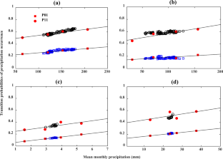
A review of recent advances in research on extreme heat events.

Climate change and variability in Kenya: a review of impacts on agriculture and food security

Extreme precipitation and temperature indices under future climate change in central Asia based on CORDEX-CORE

Data availability.

The data for ten stations are not publicly available but can be requested by contacting the corresponding author.

Brown EM, Funk CC (2008) Food security under climate change. Science 319:580–581

Article   Google Scholar  

Burn DH, Mansour R, Zhang K, Whitfield PH (2011) Trends and variability in extreme rainfall events in British Columbia. Can Water Resour J 36(1):67–82

Campbell MB et al (2016) Reducing risks to food security from climate change. Glob Food Sec 11:34–43

Cannon AJ (2018) Multivariate quantile mapping bias correction: an n-dimensional probability density function transform for climate model simulations of multiple variables. Clim Dyn 50(1–2):31–49

Chen J, Brissette FP (2014a) Comparison of five stochastic weather generators in simulating daily precipitation and temperature for the Loess Plateau of China. Int J Climatol 34:3089–3105

Chen J, Brissette F (2014b) Stochastic generation of daily precipitation amounts: review and evaluation of different models. Clim Res 59:189–206

Chen J, Zhang XC, Liu WZ, Li Z (2009) Evaluating and extending CLIGEN precipitation generation for the Loess Plateau of China. J Am Water Res Assoc 45(2):378–396

Chen J, Brissette FP, Leconte R (2011) Uncertainty of downscaling method in quantifying the impact of climate change on hydrology. J Hydrol 401:190–202

Chen J, Brissette FP, Leconte R (2012a) Coupling statistical and dynamical methods for spatial downscaling of precipitation. Clim Chang 114(3–4):509–526

Chen J, Brissette FP, Leconte R (2012b) Downscaling of weather generator parameters to quantify the hydrological impacts of climate change. Clim Res 51(3):185–200

Chen H, Xu Y, Guo S (2012c) Comparison and evaluation of multiple GCMs, statistical downscaling and hydrological models in the study of climate change impacts on runoff. J Hydrol 434–435:36–45

Chen J, Brissette FP, Leconte R, Caron A (2012d) A versatile weather generator for daily precipitation and temperature. Trans ASABE 55(3):895–906

Chen J, Brissette FP, Chaumont D, Braun M (2013a) Finding appropriate bias correction methods in downscaling precipitation for hydrologic impact studies over North America. Water Resour Res 49:4187–4205

Chen J, Brissette FP, Chaumont D, Braun M (2013b) Performance and uncertainty evaluation of empirical downscaling methods in quantifying the climate change impacts on hydrology over two North American river basins. J Hydrol 479:200–214

Chen J, Brissette FP, Leconte R (2014) Assessing regression-based statistical approaches for downscaling precipitation over North America. Hydrol Process 28(9):3482–3504

Chen J, Brissette F, Lucas-Picher P (2015) Assessing the limits of bias correcting climate model outputs for climate change impact studies. J Geophys Res Atmos 120(3):1123–1136

Chen J, Brissette FP, Liu P, Xia J (2017) Using raw regional climate model outputs for quantifying climate change impacts on hydrology. Hydrol Process 31(24):4398–4413

Chen J, Brissette FP, Caya D (2020) Remaining error sources in bias-corrected climate model outputs. Clim Chang 162:563–582

Christensen JH et al (2008) On the need for bias correction of regional climate change projections of temperature and precipitation. Geophys Res Lett 35(20):229–237

Du H, Alexander LV, Donat MG et al (2019) Precipitation from persistent extremes is increasing in most regions and globally. Geophys Res Lett 46:6041–6049

Fowler HJ et al (2007) Estimating change in extreme European precipitation using a multimodel ensemble. J Geophys Res Atmos 112(D18)

Groisman PY, Knight RW, Karl TR (2001) Heavy precipitation and high streamflow in the contiguous United States: trends in the twentieth century. Bull Am Meteorol Soc 82:219–246

Gutiérrez JM, San-Martin D, Brands S, Manzanas R, Herrera S (2013) Reassessing statistical downscaling techniques for their robust application under climate change conditions. J Clim 26:171–188

Gutiérrez JM et al (2018) An intercomparison of a large ensemble of statistical downscaling methods over Europe: results from the VALUE perfect predictor cross-validation experiment. Int J Climatol. https://doi.org/10.1002/joc.5462

Hessami M, Gachon P, Ouarda TBMJ, St-Hilaire A (2008) Automated regression-based statistical downscaling tool. Environ Model Softw 23(6):813–834

Hnilica J, Hanel M, Puš V (2017) Multisite bias correction of precipitation data from regional climate models. Int J Climatol 37(6):2934–2946

Kim BK, Kwon HH, Han D (2016) Precipitation ensembles conforming to natural variations derived from a regional climate model using a new bias correction scheme. Hydrol Earth Syst Sci 20:2019–2034

Klemeš V (1986) Operational testing of hydrological simulation models/vérification, en conditions réelles, des modèles de simulation hydrologique. Hydrol Sci J 31:13–24

Manzanas R, Fiwa L, Vanya C, Kanamaru H, Gutiérrez JM (2020) Statistical downscaling or bias adjustment? A case study involving implausible climate change projections of precipitation in Malawi. Clim Chang 162:1437–1453

Maraun D (2012) Nonstationarities of regional climate model biases in European seasonal mean temperature and precipitation sums. Geophys Res Lett 39:L06706

Maraun D et al (2010) Precipitation downscaling under climate change: recent developments to bridge the gap between dynamical models and the end user. Rev Geophys 48(3):RG3003 8755–1209

Mpelasoka FS, Chiew FHS (2009) Influence of rainfall scenario construction methods on runoff projections. J Hydrometeorol 10(5):1168–1183

Mullan D, Chen J, Zhang XC (2016) Validation of non-stationary precipitation series for site-specific impact assessment: comparison of two statistical downscaling techniques. Clim Dyn 46(3):967–986

Murphy J (1999) An evaluation of statistical and dynamical techniques for downscaling local climate. J Clim 12(8):2256–2284

Nash JE, Sutcliffe WH (1970) River flow forecasting through conceptual models: part 1. A discussion of principles. J Hydrol 10:282–290

Nikulin G, Asharaf S, Magariño ME et al (2018) Dynamical and statistical downscaling of a global seasonal hindcast in eastern Africa. Clim Serv 9:72–85

Polade SD, Pierce DW, Cayan DR, Gershunov A, Dettinger MD (2014) The key role of dry days in changing regional climate and precipitation regimes. Sci Rep 4:1–8

Google Scholar  

Qian BD, Gameda S, Jong R, Fallon P, Gornall J (2010) Comparing scenarios of Canadian daily climate extremes derived using a weather generator. Clim Res 41(2):131–149

Schmidli J, Frei C, Vidale PL (2006) Downscaling from GCM precipitation: a benchmark for dynamical and statistical downscaling methods. Int J Climatol 26:679–689

Seager R et al (2007) Model projections of an imminent transition to a more arid climate in southwestern North America. Science 316:1181–1184

Teutschbein C, Seibert J (2013) Is bias correction of regional climate model (RCM) simulations possible for non-stationary conditions? Hydrol Earth Syst Sci 17:5061–5077

Themeßl MJ, Gobiet A, Heinrich G (2012) Empirical-statistical downscaling and error correction of regional climate models and its impact on the climate change signal. Clim Chang 112(2):449–446

Toride K, Cawthorne DL, Ishida K, Kavvas ML, Anderson ML (2018) Long-term trend analysis on total and extreme precipitation over Shasta Dam watershed. Sci Total Environ 626:244–254

Vaghefi P, Yu B (2011) Use of CLIGEN to simulate climate change in southeastern Australia. Trans ASABE 54(3):857–867

van Roosmalen L, Christensen JH, Butts MB, Jensen KH, Refsgaard JC (2010) An intercomparison of regional climate model data for hydrological impact studies in Denmark. J Hydrol 380(3–4):406–419

Vrac M, Friederichs P (2015) Multivariate—intervariable, spatial, and temporal—bias correction. J Clim 28(1):218–237

Wilby RL, Hay LE, Leavesley GH (1999) A comparison of downscaled and raw GCM output: implications for climate change scenarios in the San Juan River Basin, Colorado. J Hydrol 225:67–91

Wilby RL, Dawson CW, Barrow EM (2002) SDSM—a decision support tool for the assessment of regional climate change impacts. Environ Model Softw 17(2):147–159

Wilks DS (1992) Adapting stochastic weather generation algorithms for climate change studies. Clim Chang 22(1):67–84

Wilks DS (1999) Interannual variability and extreme-value characteristics of several stochastic daily precipitation models. Agric For Meteorol 93:153–169

Xu CY (1999) From GCMs to river flow: a review of downscaling methods and hydrologic modelling approaches. Prog Phys Geogr 23(2):229–249

Yeh H-F, Hsu H-L (2019) Using the Markov chain to analyze precipitation and groundwater drought characteristics and linkage with atmospheric circulation. Sustainability 11:1817. https://doi.org/10.3390/su11061817

Yu B (2005) Adjustment of CLIGEN parameters to generate precipitation change scenarios in southeastern Australia. Catena 61(2–3):196–209

Zhang XC (2005) Spatial downscaling of global climate model output for site-specific assessment of crop production and soil erosion. Agric For Meteorol 135:215–229

Zhang XC (2013a) Verifying a temporal disaggregation method for generating daily precipitation of potentially non-stationary climate change for site-specific impact assessment. Int J Climatol 33:326–342

Zhang XC (2013b) Adjusting skewness and maximum 0.5-hour intensity in CLIGEN to improve extreme event and sub-daily intensity generation for assessing climate change impacts. Trans ASABE 56(5):1703–1713

Zhang XC, Garbrecht JD (2003) Evaluation of CLIGEN precipitation parameters and their implication on WEPP runoff and erosion prediction. Trans ASAE 46(2):311–320

Zhang XC, Chen J, Garbrecht JD, Brissette FP (2012) Evaluation of a weather generator-based method for statistically downscaling nonstationary climate scenarios for impact assessment at a point scale. Trans ASABE 55(5):1745–1756

Download references

Acknowledgements

The authors like to express great appreciation to Dr. Bofu Yu of Griffith University, Australia, for providing daily precipitation data of the Cataract Dam and Port Macquarie stations; to Dr. Alfredo Borges de Campos of Universidade Federal de Goias, Brazil, for data of the Campinas station; and to Dr. Donal Mullan of Queen’s University Belfast, UK, for data of the Armagh and Durham stations.

Code availability

The custom code was only used for calculations, and it can be provided by contacting the corresponding author.

This work was partially supported by the National Natural Science Foundation of China (Grant No. 52079093; 51779176), the Hubei Provincial Natural Science Foundation of China (Grant No. 2020CFA100), and the Overseas Expertise Introduction Project for Discipline Innovation (111 Project) funded by the Ministry of Education and State Administration of Foreign Experts Affairs P.R. China (Grant No. B18037).

Author information

Authors and affiliations.

State Key Laboratory of Water Resources & Hydropower Engineering Science, Wuhan University, 299 Bayi Road, Wuchang Distinct, Wuhan, 430072, Hubei, China

USDA-ARS, Grazinglands Research Laboratory, 7207W. Cheyenne St., El Reno, OK, 73036, USA

Xunchang John Zhang

You can also search for this author in PubMed   Google Scholar

Contributions

JC and XJZ conceived the original idea, designed the methodology, and collected the data. JC developed the model code and performed the simulations. JC and XJZ contributed to the interpretation of results. JC wrote the paper, and XJZ revised the paper.

Corresponding author

Correspondence to Jie Chen .

Ethics declarations

Conflict of interest.

The authors declare no competing interests.

Additional information

Publisher’s note.

Springer Nature remains neutral with regard to jurisdictional claims in published maps and institutional affiliations.

Supplementary information

(DOCX 1602 kb)

Rights and permissions

Reprints and permissions

About this article

Chen, J., Zhang, X.J. Challenges and potential solutions in statistical downscaling of precipitation. Climatic Change 165 , 63 (2021). https://doi.org/10.1007/s10584-021-03083-3

Download citation

Received : 15 May 2020

Accepted : 30 March 2021

Published : 24 April 2021

DOI : https://doi.org/10.1007/s10584-021-03083-3

Share this article

Anyone you share the following link with will be able to read this content:

Sorry, a shareable link is not currently available for this article.

Provided by the Springer Nature SharedIt content-sharing initiative

• Statistical downscaling
• Temporal sequence of precipitation
• Daily precipitation extreme
• Nonstationarity
• Find a journal
• Publish with us
• Track your research

Generative diffusion-based downscaling for climate

Downscaling, or super-resolution, provides decision-makers with detailed, high-resolution information about the potential risks and impacts of climate change, based on climate model output. Machine learning algorithms are proving themselves to be efficient and accurate approaches to downscaling. Here, we show how a generative, diffusion-based approach to downscaling gives accurate downscaled results. We focus on an idealised setting where we recover ERA5 at 0.25 ⁢ ° 0.25 ° 0.25\degree 0.25 °  resolution from coarse grained version at 2 ⁢ ° 2 ° 2\degree 2 °  resolution. The diffusion-based method provides superior accuracy compared to a standard U-Net, particularly at the fine scales, as highlighted by a spectral decomposition. Additionally, the generative approach provides users with a probability distribution which can be used for risk assessment. This research highlights the potential of diffusion-based downscaling techniques in providing reliable and detailed climate predictions.

K eywords  Diffusion   ⋅ ⋅ \cdot ⋅ Generative models   ⋅ ⋅ \cdot ⋅ Machine learning   ⋅ ⋅ \cdot ⋅ Climate models   ⋅ ⋅ \cdot ⋅ Downscaling   ⋅ ⋅ \cdot ⋅ Super-resolution

1 Introduction

Climate change poses a threat to humans and ecosystems all over the world. The potential impacts range from increased risk of damage caused by extreme events such as heatwaves, heavy rainfall, and flooding events, to disruptions in biodiversity, agriculture, and threats to food security. This underscores the critical need for accurate predictions of future climate conditions for effective mitigation and adaptation strategies.

Global Climate Models (GCMs) have been pivotal in our efforts to simulate the Earth’s complex system and project future climate scenarios. GCMs are sophisticated computer models that incorporate components from the atmosphere, ocean, land, vegetation, and sea-ice, creating a coupled Earth system. However, the computational cost associated with running GCMs at high resolutions presents a significant challenge. Currently, GCMs operate on a grid with a typical resolution of approximately 1 ⁢ ° 1 ° 1\degree 1 ° (roughly 100 kilometers) [ Chen et al., 2021b ] . For assessing climate change impacts, we often require more localised predictions, crucial for addressing regional impacts. This limitation prompts the exploration of alternative methodologies, such as downscaling, to enhance the spatial precision of climate predictions.

In recent years, machine learning techniques have proven capable of making substantial strides in predicting climate patterns. Many believe it will revolutionise our approach to climate modeling, by offering computationally efficient methods to improve, or even replace, traditional GCMs [ Balaji, 2021 , Schneider et al., 2023 , Mansfield et al., 2023 , Rolnick et al., 2023 ] . The challenges of climate and weather prediction have caught the attention of large technology companies, such as Google, NVIDIA, Microsoft, Huawei, and others, who are leveraging machine learning to facilitate numerical weather prediction [ Lam et al., 2023 , Pathak et al., 2022 , Bi et al., 2022 , Nguyen et al., 2023 , Chen et al., 2023 ] . There is also a growing interest in machine learning emulators of GCMs [ Mansfield et al., 2020 , Watson, 2022 , Watt-Meyer et al., 2023 ] and in embedding machine learning components into GCMs (such as subgrid-scale parameterisations) [ Kochkov et al., 2024 , O’Gorman and Dwyer, 2018 , Gentine et al., 2018 ] , amongst other uses [ Molina et al., 2023 ] .

One specific avenue gaining popularity is downscaling, a technique where coarse-resolution climate models are refined using machine learning to generate high-resolution predictions. This could enhance the cost-effectiveness of coarse climate models and their precision on regional scales. This paper uses a generative machine learning approach based on diffusion [ Sohl-Dickstein et al., 2015 ] for downscaling climate data. Using the ERA5 reanalysis dataset, we show how a diffusion models can enhance a coarse resolution map of temperature and winds over the USA [ Hersbach et al., 2020 ] . The benefit is that ensembles can be produced, which are crucial for assessing model uncertainty in climate change studies [ Hawkins and Sutton, 2009 ] . Diffusion-based generative models have been applied in similar downscaling applications [ Mardani et al., 2023 , Addison et al., 2022 , Nath et al., 2024 ] , although they have not yet gained prominence in the climate downscaling literature. Our aim is to contribute to the evolving landscape of machine learning climate downscaling, with a diffusion-based approach applied on continental scales for one of the first times. While previous studies focus on downscaling to km-scale resolution [ Mardani et al., 2023 , Addison et al., 2022 , Nath et al., 2024 ] , we envision how diffusion could be used to downscale conventional climate models with typical CMIP-resolution, i.e., 𝒪 ( \mathcal{O}( caligraphic_O ( 1° ) ) ) ) or 𝒪 ⁢ ( 100 ⁢  km ) 𝒪 100  km \mathcal{O}(100\mbox{ km}) caligraphic_O ( 100 km ) , to a higher resolution that would typically require a regional climate model, i.e., 𝒪 ( \mathcal{O}( caligraphic_O ( 0.1° ) ) ) ) or 𝒪 ⁢ ( 10 ⁢  km ) 𝒪 10  km \mathcal{O}(10\mbox{ km}) caligraphic_O ( 10 km ) . In agreement with several recent studies, our results show that diffusion-based generative models are a promising approach for climate data, both for downscaling [ Mardani et al., 2023 , Addison et al., 2022 , Nath et al., 2024 ] and in other applications [ Huang et al., 2024 , Price et al., 2023 , Chan et al., 2024 , Bassetti et al., 2023 , Cachay et al., 2023 ] .

2 Background

2.1 downscaling.

Climate downscaling, often referred to as super-resolution (based on the machine vision literature), is the process of refining predictions from a low-resolution climate model to a higher resolution. This step is crucial for addressing the limitations of global climate models (GCMs) and tailoring climate predictions to local or regional scales. Traditionally, two main approaches have been employed for downscaling: dynamical downscaling and statistical downscaling, where the latter includes machine learning techniques growing in popularity recently.

Dynamical downscaling involves running a regional climate model (RCM) at a higher resolution, typically 10-50 km, over a specific region of interest [ Sunyer et al., 2012 , Giorgi, 2019 , Tapiador et al., 2020 , Giorgi and Jr, 2015 ] . The low-resolution output from a GCM serves as both the boundary and initial conditions for the RCM. RCMs offer the advantage of enhanced spatial resolution, while guaranteeing the output is dynamically consistent, rendering them popular amongst stakeholders and policymakers for important decisions [ Gutowski et al., 2020 ] . However, RCMs also have inherent biases, like GCMs, and may still require postprocessing techniques to remove biases. Importantly, dynamical downscaling comes with a notable drawback in the high computational cost of running high-resolution RCMs.

Statistical downscaling , in contrast, utilises statistical methods to establish relationships between coarse-resolution model outputs and high-resolution observations in historical data [ Maraun and Widmann, 2018b , Vandal et al., 2019 ] . One approach is to employ a regression model which directly predicts high resolution model variables from low resolution model variables. This assumes that the low resolution model is a “perfect” predictor of the high resolution model (i.e., there are no model biases). This is traditionally known as “perfect prognosis” [ Schubert, 1998 ] . Since low resolution models are often missing processes and feedbacks, this approach alone can lead to inaccurate downscaled predictions [ Maraun and Widmann, 2018a ] . An alternative approach, known as “model output statistics”, aims to match the predicted statistics to observed statistics, such as the mean, standard deviation, and/or quantiles. This automatically accounts for model biases and is used for the NASA Earth Exchange Global Daily Downscaled Projections [ Thrasher et al., 2022 ] . Another approach lies in “stochastic weather generators”, that simulate stochasticity of weather data based on characteristics of observations [ Wilby et al., 1998 ]

Although faster than dynamical downscaling, these traditional methods often exhibit poor performance in extrapolating to new climates. This limitation arises from the assumption that the same statistical relationships hold under changing conditions, known as stationarity, which we cannot necessarily expect to be true [ Fowler et al., 2007 , Maraun et al., 2017 ] . One solution could be hybrid downscaling, such as statistical downscaling applied to RCM outputs [ Sunyer et al., 2012 ] . Alternatively, machine learning/artificial intelligence may offer solutions to this problem.

Machine learning techniques are becoming a popular choice for statistical downscaling that can be framed as perfect prognosis [ Baño-Medina et al., 2022 ] , model output statistics [ Pour et al., 2018 ] , weather generators [ Wilby et al., 1998 ] or a combination of these [ Vandal et al., 2019 ] . Many of these approaches are based on developments in computer vision for super-resolution of images [ Glasner et al., 2009 ] .

2.2 Machine learning

Downscaling can be viewed as a supervised learning task, where the goal is to learn the variables on the high resolution grid (the target), from the variables on the low resolution grid (the input). The majority of machine learning studies aim to directly learn the mapping between the low resolution input and the high resolution target with a wide variety of machine learning architectures, including random forests [ Hasan Karaman and Akyürek, 2023 , Medrano et al., 2023 , Chen et al., 2021a ] , support vector machines [ Pour et al., 2018 ] , and convolutional neural network (CNN) architectures [ Baño-Medina et al., 2022 , Jiang et al., 2021 , Wang et al., 2019 ] , including U-Net architectures [ Agrawal et al., 2019 , Kaparakis and Mehrkanoon, 2023 , Adewoyin et al., 2021 , Cho et al., 2023 ] , convolutional autoencoders [ Babaousmail et al., 2021 ] and fourier neural operators [ Yang et al., 2023 ] . These studies show that machine learning can be more accurate than conventional statistical downscaling, with the benefit of low computational cost compared against dynamical downscaling approaches. However, end-users are often concerned when there is a risk of unrealistic predictions from black-box machine learning methods, especially when used in new scenarios such as climate change. Recently, physics-informed machine learning has shown to be a potential solution to this, by embedding known constraints from physics [ Harder et al., 2024 , Harder et al., 2022 ] .

Generative models , which aim to learn underlying probabilities distributions of the data, are a promising approach for matching downscaled statistics to that of observations (similar to statistical downscaling with “model output statistics” described above). Many high resolution images can be generated through sampling, or conditioning on , the low resolution data (also making them a type of “stochastic weather generator”). For example, several recent studies use Generative Adverserial Networks (GANs) to generate high resolution images conditioned on low resolution images [ Leinonen et al., 2021 , Harris et al., 2022 , Oyama et al., 2023 , Wang et al., 2021 , Price and Rasp, 2022 ] . Diffusion-based approaches have become established as a state-of-the-art technique for image generation (e.g., Stable Diffusion [ Rombach et al., 2022 ] , DALL-E2 [ Ramesh et al., 2022 ] , amongst others [ Saharia et al., 2022 , Nichol et al., 2022 ] ) but have not yet become widely used for climate downscaling. We expect to see more diffusion-based downscaling methods in the near future, following [ Bischoff and Deck, 2023 , Wan et al., 2023 ] who used diffusion for downscaling turbulent fluid data and [ Mardani et al., 2023 , Addison et al., 2022 , Nath et al., 2024 ] who presented diffusion for downscaling climate model output on localised scales. In a similar realm, [ Groenke et al., 2020 ] use unsupervised normalising flows to downscale climate variables. In this study, we demonstrate the performance of a diffusion-based approach to downscaling on a continental scale.

The probabilistic nature of generative machine learning makes them particularly desirable for risk assessment studies, such as those aiming to quantify the likelihood of extreme events. Both weather and climate modelling communities have long used ensembles of simulations to assess model, scenario, and initial condition uncertainty [ Hawkins and Sutton, 2009 ] . There is a growing interest in generative machine learning for generating ensembles from one climate/weather model simulation [ Li et al., 2023 ] . In a downscaling setting, ensembles could be leveraged to determine the trustworthiness of predictions, for example, by highlighting increased model uncertainty when applied to out-of-distribution samples that are likely to occur in a non-stationary climate [ Fowler et al., 2007 ] .

The ERA5 reanalysis dataset , made publicly available by ECMWF [ Hersbach et al., 2020 ] , is used in this study. Reanalysis datasets optimally combine observations and models through data assimilation techniques. ERA5 includes hourly estimates for a wide range of atmospheric, land, and oceanic climate variables on a 0.25 ⁢ ° 0.25 ° 0.25\degree 0.25 °  resolution longitude-latitude grid with 137 vertical levels, from January 1940 to present day. This dataset is becoming widely used in other machine learning weather/climate prediction studies [ Pathak et al., 2022 , Bi et al., 2022 , Lam et al., 2023 , Chen et al., 2023 ] .

We consider downscaling of three variables over the continental USA:

Air temperature at 2 m

Zonal wind at 100 m

Meridional wind at 100 m

We focus only on these three variables over the USA as a demonstration of diffusion for downscaling on continental scales. Although relevant for extreme events, we do not include precipitation here because because ERA5 reanalysis at 0.25 ⁢ ° 0.25 ° 0.25\degree 0.25 ° resolution is likely too coarse to capture its spatial intermittency [ Bihlo, 2021 ] . Diffusion-based approaches to downscaling precipitation on kilometer scales can be found in [ Mardani et al., 2023 , Harris et al., 2022 , Nath et al., 2024 ] .

ERA5 provides hourly data from 1940 to present day, however, we expect this to be highly correlated in the temporal domain. To reduce the dataset size without significant loss of information, we subsample randomly in time to select only 30 timesteps per month. This reduces the dataset size by 1 / 24 1 24 1/24 1 / 24 and gives us data sampled approximately once per day, at different times of day. We use years 1950-2022 and separate this into a training dataset (1950-2017) and testing dataset (2018-2022).

We aim to downscale a coarsened version of the ERA5 dataset back onto the original 0.25 ⁢ ° 0.25 ° 0.25\degree 0.25 °  resolution grid. For the coarsened dataset, we use bi-linear interpolation onto a 2 ⁢ ° 2 ° 2\degree 2 °  resolution grid, to be approximately consistent with typical climate model resolution (e.g., 𝒪 ⁢ ( 1 ⁢ ° ) 𝒪 1 ° \mathcal{O}(1\degree) caligraphic_O ( 1 ° ) in CMIP6 models [ Chen et al., 2021b ] ). This corresponds to approximately 8 × 8\times 8 × scaling of resolution. Note that this approach assumes the coarse resolution data is not biased, following the perfect prognosis approach to downscaling. To apply this to real climate model data, one may first need to carry out bias correction [ Mardani et al., 2023 ] .

3.2 Baseline U-Net for downscaling

Our problem is a supervised learning problem, where we aim to learn the fine resolution variables from the coarse resolution variables. We will compare two approaches for this task: firstly, a U-Net architecture and secondly, a diffusion-based generative model. Since the inputs and outputs are both images with a channel for each variable, this requires an image-to-image model such as a U-Net [ Ronneberger et al., 2015 ] . A U-Net architecture is a neural network comprised of several encoding convolutional layers followed by several decoding up-convolutional layers, making them ideal for computer vision tasks when the input and output images are of the same size. They have shown excellent performance on image processing tasks, such as segmentation [ Ronneberger et al., 2015 ] and and super-resolution [ Hu et al., 2019 ] . As we will see in the following section, our diffusion-based approach also uses a U-Net, allowing us to use the same base model, making for a fair comparison between these methods.

Our input variables are the air temperature at 2 m, and zonal and meridional winds at 100 m, all coarsened onto the 2 ⁢ ° 2 ° 2\degree 2 °  resolution grid. Note that after coarsening, these variables are stored on the fine resolution ( 0.25 ⁢ ° 0.25 ° 0.25\degree 0.25 ° ) grid using bi-linear interpolation, ensuring that the inputs and outputs have the same dimensions and allowing for a simple U-Net architecture. To improve efficiency of the U-Net, rather than directly learning the output on the fine resolution grid, we learn the difference between the output on the fine and coarse grid. As well as these inputs, we also provide the U-Net with fixed inputs for spatial quantities that describe the geography and are constant in time. These are the land-sea mask and the height of the land surface, defined on the fine resolution grid. We expect these to aid learning of details around the coast, the great lakes and the mountains. This means the input image is of size (128 x 256 x 5) while the output image is of size (128 x 256 x 3). Finally, we also provide scalar values representing the month and the time of day, allowing the U-Net to learn differences in the diurnal and seasonal cycles. These are input to the each block of the U-Net, using a shallow neural network. Table  1 shows these inputs and outputs to the network. All variables are normalised to have standard scaling with zero mean and unit variance. The U-Net is trained by minimising the Mean Squared Error (MSE) between the U-Net predicted image and the samples from the data.

3.3 Diffusion-based generative model

Generative models using diffusion have shown great success as a method for synthesising images [ Sohl-Dickstein et al., 2015 ] . As a generative model, the goal is to learn some probability distribution p ⁢ ( 𝐱 ) 𝑝 𝐱 p(\mathbf{x}) italic_p ( bold_x ) given a set of samples { 𝐱 } 𝐱 \{\mathbf{x}\} { bold_x } . This would be an unconditional model, however, we are interested in building a conditional model, p ⁢ ( 𝐱 | 𝐲 ) 𝑝 conditional 𝐱 𝐲 p(\mathbf{x}|\mathbf{y}) italic_p ( bold_x | bold_y ) , where 𝐱 𝐱 \mathbf{x} bold_x are the high resolution image samples and 𝐲 𝐲 \mathbf{y} bold_y are the low resolution image samples. In the following discussion, we will neglect the conditioning on 𝐲 𝐲 \mathbf{y} bold_y for clarity, but note that the conditional form is obtained by replacing 𝐱 𝐱 \mathbf{x} bold_x with 𝐱 | 𝐲 conditional 𝐱 𝐲 \mathbf{x}|\mathbf{y} bold_x | bold_y .

Diffusion models take inspiration from thermodynamics whereby a diffusion process { 𝐱 ⁢ ( t ) } t = 0 T subscript superscript 𝐱 𝑡 𝑇 𝑡 0 \{\mathbf{x}(t)\}^{T}_{t=0} { bold_x ( italic_t ) } start_POSTSUPERSCRIPT italic_T end_POSTSUPERSCRIPT start_POSTSUBSCRIPT italic_t = 0 end_POSTSUBSCRIPT with t ∈ [ 0 , T ] 𝑡 0 𝑇 t\in[0,T] italic_t ∈ [ 0 , italic_T ] is constructed which transforms samples from the data distribution 𝐱 ⁢ ( 0 ) ∼ p ⁢ ( 𝐱 ) similar-to 𝐱 0 𝑝 𝐱 \mathbf{x}(0)\sim p(\mathbf{x}) bold_x ( 0 ) ∼ italic_p ( bold_x ) to that of an isotropic Gaussian 𝐱 ⁢ ( T ) ∼ 𝒩 ⁢ ( 𝟎 , σ ⁢ 𝐈 ) similar-to 𝐱 𝑇 𝒩 0 𝜎 𝐈 \mathbf{x}(T)\sim\mathcal{N}(\mathbf{0},\sigma\mathbf{I}) bold_x ( italic_T ) ∼ caligraphic_N ( bold_0 , italic_σ bold_I ) . Following [ Song et al., 2021 ] , the stochastic differential equation for such a process is given by

where 𝐟 ⁢ ( 𝐱 , t ) 𝐟 𝐱 𝑡 \mathbf{f}(\mathbf{x},t) bold_f ( bold_x , italic_t ) is the drift coefficient g ⁢ ( t ) 𝑔 𝑡 g(t) italic_g ( italic_t ) is the diffusion coefficient and 𝐰 𝐰 \mathbf{w} bold_w is a Wiener process. If this process can be reversed, one can use it to generate samples from p ⁢ ( 𝐱 0 ) 𝑝 subscript 𝐱 0 p(\mathbf{x}_{0}) italic_p ( bold_x start_POSTSUBSCRIPT 0 end_POSTSUBSCRIPT ) . This involves first sampling from the terminal distribution 𝐱 ⁢ ( T ) 𝐱 𝑇 \mathbf{x}(T) bold_x ( italic_T ) (the isotropic Gaussian), then transforming the sample through the reverse processes to the data distribution. It can be shown that the reverse of a diffusion process is itself a diffusion process with the following reverse time stochastic differential equation (SDE) [ Anderson, 1982 ]

where 𝐰 ¯ ¯ 𝐰 \overline{\mathbf{w}} over¯ start_ARG bold_w end_ARG is a Wiener process with time flowing backwards from T to 0. ∇ 𝐱 log ⁢ p t ⁢ ( 𝐱 ) subscript ∇ 𝐱 log subscript 𝑝 𝑡 𝐱 \nabla_{\mathbf{x}}\mathrm{log}p_{t}(\mathbf{x}) ∇ start_POSTSUBSCRIPT bold_x end_POSTSUBSCRIPT roman_log italic_p start_POSTSUBSCRIPT italic_t end_POSTSUBSCRIPT ( bold_x ) is the score function, a vector field which points towards higher density. The score does not depend on the intractable normalisation constant making it easier to evaluate. Obtaining samples by solving the reverse SDE requires knowledge of the score function. To do this we parameterise the score using a neural network 𝐬 θ ⁢ ( 𝐱 , t ) subscript 𝐬 𝜃 𝐱 𝑡 \mathbf{s}_{\mathbf{\theta}}(\mathbf{x},t) bold_s start_POSTSUBSCRIPT italic_θ end_POSTSUBSCRIPT ( bold_x , italic_t ) , with the same U-Net architecture as described above in Section 3.2 . The weights of 𝐬 θ ⁢ ( 𝐱 , t ) subscript 𝐬 𝜃 𝐱 𝑡 \mathbf{s}_{\mathbf{\theta}}(\mathbf{x},t) bold_s start_POSTSUBSCRIPT italic_θ end_POSTSUBSCRIPT ( bold_x , italic_t ) are optimised using score matching [ Vincent, 2011 ] by minimising the following loss [ Song et al., 2021 ]

where λ ⁢ ( t ) 𝜆 𝑡 \lambda(t) italic_λ ( italic_t ) is a weighting function, t is sampled uniformly between [ 0 , T ] 0 𝑇 [0,T] [ 0 , italic_T ] . This equation is obtained through minimising the evidence lower bound (ELBO) on the negative log likelihood, 𝔼 ⁢ [ − log ⁢ p ⁢ ( 𝐱 0 ) ] 𝔼 delimited-[] log 𝑝 subscript 𝐱 0 \mathbb{E}[-\mathrm{log}\,p(\mathbf{x}_{0})] blackboard_E [ - roman_log italic_p ( bold_x start_POSTSUBSCRIPT 0 end_POSTSUBSCRIPT ) ] , and reweighting by λ ⁢ ( t ) 𝜆 𝑡 \lambda(t) italic_λ ( italic_t ) .

Within the framework discussed above, there are a number of design choices and free parameters to set. In this work, we use the implementation given by Karras et al [ Karras et al., 2022 ] . Their suggestions give a noticeable improvement over previous works [ Song et al., 2021 , Ho et al., 2020 , Nichol and Dhariwal, 2021 ] for image synthesis. One improvement to note is the use of a higher order (second) integration scheme. This significantly reduces the number of timesteps taken when solving the reverse process making inference significantly more efficient. We use 100 timesteps during evaluation, but find that using just 50 is sufficient for a similar accuracy.

After training on years 2050-2017 of ERA5, we evaluate the performance of both the U-Net and the diffusion-based model on years 2018-2022.

4.1 Example

Figure 1 shows the coarse resolution maps, the true fine resolution maps, and the downscaled fine resolution maps for the U-Net and diffusion, for one snapshot for all three variables. Both machine learning approaches demonstrate good predictions when compared against the fine resolution. For temperature, the U-Net and diffusion predictions are virtually indistinguishable. For the winds, there are some smaller scale features in the diffusion prediction, while the U-Net predicts smoother features. We expect this is because U-Net is trained to minimise MSE, which naturally favours smoother fields rather than high frequency variations.

4.2 Probabilistic Predictions

Figure 1 (j-l), shows one generated downscaled prediction from the diffusion model. However, one of the benefits of the diffusion-based model lies in its ability to generate multiple predictions, creating probability distributions, rather than one deterministic prediction. We generate an ensemble of diffusion predictions consisting of 30 samples, each of which is generated from a different sample from the terminal Gaussian distribution 𝐱 ⁢ ( T ) 𝐱 𝑇 \mathbf{x}(T) bold_x ( italic_T ) . This provides us with valuable information when making high-stakes decisions, for example, by highlighting when there is higher uncertainty amongst ensemble members. We find the ensemble members agree reasonably well and show their 1 standard deviation in Figure 1 (m-n) for each variable. There is higher uncertainty in regions where the variable is changing quickly, in other words, where there are larger spatial gradients. For the surface temperatures, this increased uncertainty tends to be over mountainous regions and for the winds, to the east of mountains and along fronts where the winds are rapidly changing. This makes sense for a downscaling problem where the prediction is constrained by the coarse grid, but the diffusion generates many possible realisations for how the variables could be interpolated between the coarse grid cells. This also results in a gridded pattern where predictions closer to the coarse grid cells have lower uncertainty.

4.3 Metrics

Here, we aim to compare the results of a deterministic U-Net with a probabilistic diffusion-based model. To compare both, we will use the mean absolute error (MAE). For the diffusion-based model, we use the mean across across the ensemble. To consider the probabilistic nature of diffusion, we will also consider the continuous ranked probability score (CRPS), a generalisation of mean absolute error to compare predicted probability distributions to a single ground truth [ Hersbach, 2000 , Gneiting and Raftery, 2007 ] . Note, that we present the CRPS metric for diffusion only and cannot fairly compare this with the deterministic U-Net predictions.

Figure 2 shows maps showing these metrics averaged over the entire test dataset. The gridded pattern appears due to reduced error at grid-cells close to the coarse-reoslution grid, also present in Figure 1 (m-o). The diffusion-based approach shows slightly lower MAE in the high altitude regions along the Rockies, particularly for temperature. These are the regions that exhibit more variability, both in time and space, which could explain why a probablistic model performs better. The value in the probabilistic approach is further highlighted by the significant reduction in error when considering the CRPS metric for diffusion, which takes into account all ensemble members.

Table 2 shows the mean metrics, averaged across the entire domain and test dataset. Note that when taking spatial averages, we weight each grid-cell by the cosine of latitude to account for the non-uniform size of grid cells.

4.4 Spectra

In the example snapshots (Figure 1 ), it appears that the diffusion model produces more accurate high frequency variations for the winds compared to the U-Net. We validate this further by calculating the power spectra across all wavelengths, for all three variables. Here, we treat the data as an image and take a 2D Fourier transform across this image to estimate the power for each wavelength. These results are robust to transforming the data onto a grid equispaced in distance, accounting for different grid spacing in latitude.

Figure 3 (a-c) shows the power spectra for each variable for all methods on a log-scale, compared against the ground truth in black. The power spectra for diffusion is indistinguishable from the ground truth, so we also present the differences between these in Figure 3 (d-f). The power spectra is significantly more accurate across all scales in the diffusion model in comparison to the U-Net. For the winds, we see this is more evident at the high wavenumbers. This shows the promise of diffusion for approximating geospatial data for a range of uses, potentially addressing issues of oversmoothing seen in other weather and climate studies [ Pathak et al., 2022 , Bi et al., 2022 , Lam et al., 2023 ] .

5 Conclusions

In this paper, we have presented a generative diffusion-based model for downscaling climate data on continental scales. We demonstrated this by recovering 0.25 ⁢ ° 0.25 ° 0.25\degree 0.25 °  resolution ERA5 data from a 2 ⁢ ° 2 ° 2\degree 2 °  resolution coarse-grained version of ERA5 and found that the diffusion model outperformed a baseline U-Net with the same architecture. The next step would be to apply this diffusion model to downscale the output of a coarse 𝒪 ( \mathcal{O}( caligraphic_O ( 1° ) ) ) )  resolution climate model to a higher resolution, e.g., 0.25 ⁢ ° 0.25 ° 0.25\degree 0.25 °  ERA5. This presents the additional challenge that the coarse model output may not match up with the high resolution dataset. One approach could be to first apply a bias-correction technique, as done in [ Mardani et al., 2023 ] . The application of downscaling to climate model output based on historical observational datasets also presents the issue of non-stationarity, whereby we cannot assume that the relationship between the coarse resolution and the high resolution data remains constant under a changing climate. Diffusion-based approaches may be appealing for this task, as they predict an ensemble which can highlight the epistemic uncertainty associated with each prediction.

There are a wide range of avenues to expand upon this study, for example, increasing the number of variables predicted, exploring performance at different resolutions, applying the same method to different regions or to full global data, or incorporating temporal, as well as spatial, downscaling. Downscaling of precipitation is of particular interest, due to its intermittent spatial patterns that is typically overly smooth in climate model output compared to observations and is a crucial variable for extreme events such as flooding [ Sunyer et al., 2012 , Baño-Medina et al., 2022 , Vandal et al., 2017 , Xu et al., 2020 , Akinsanola et al., 2018 , Babaousmail et al., 2021 , Harris et al., 2022 ] .

This study was carried out without access to expensive, high performance computing systems. Although both training and inference was more expensive than the baseline U-Net, diffusion offers significantly improved performance and the ability to generate ensembles, with a computational cost several orders of magnitude lower than full climate model simulations. This could make impact studies accessible and affordable to a wider range of end-users. We conclude this study by noting that, given the rapid improvements in diffusion-based image generation in the last three years [ Zhang et al., 2023 ] , we might expect to see even more advances in diffusion-based techniques applied to climate problems. Even during the time it took us to complete this study, we have seen diffusion models gaining popularity in this field [ Mardani et al., 2023 , Price et al., 2023 , Nath et al., 2024 , Huang et al., 2024 , Chan et al., 2024 ] , a trend that we hope will continue in the years to come.

Open data statement

All code used in this study is available at https://github.com/robbiewatt1/ClimateDiffuse . We followed the diffusion implementation of [ Karras et al., 2022 ] available at https://github.com/NVlabs/edm . The ERA5 reanalysis dataset used in this study is publicly available at https://cds.climate.copernicus.eu/cdsapp#!/dataset/reanalysis-era5-complete?tab=overview [ Hersbach et al., 2020 ] .

Acknowledgements

This was done in our spare time and not directly funded. We acknowledge our employer, Stanford University, for support and access to journal articles. LAM would also like to acknowledge support from Schmidt Sciences, that funds her research at the intersection of machine learning and climate modeling.

• [Addison et al., 2022] Addison, H., Kendon, E., Ravuri, S., Aitchison, L., and Watson, P. A. (2022). Machine learning emulation of a local-scale UK climate model. arXiv:2211.16116 [physics].
• [Adewoyin et al., 2021] Adewoyin, R. A., Dueben, P., Watson, P., He, Y., and Dutta, R. (2021). TRU-NET: a deep learning approach to high resolution prediction of rainfall. Machine Learning , 110(8):2035–2062.
• [Agrawal et al., 2019] Agrawal, S., Barrington, L., Bromberg, C., Burge, J., Gazen, C., and Hickey, J. (2019). Machine Learning for Precipitation Nowcasting from Radar Images. arXiv:1912.12132 [cs, stat].
• [Akinsanola et al., 2018] Akinsanola, A., Ajayi, V., Adejare, A., Adeyeri, O., Gbode, I., Ogunjobi, K., Nikulin, G., and Abolude, A. (2018). Evaluation of rainfall simulations over West Africa in dynamically downscaled CMIP5 global circulation models. Theoretical and Applied Climatology , 132(1):437–450.
• [Anderson, 1982] Anderson, B. D. O. (1982). Reverse-time diffusion equation models. Stochastic Processes and their Applications , 12(3):313–326.
• [Babaousmail et al., 2021] Babaousmail, H., Hou, R., Gnitou, G. T., and Ayugi, B. (2021). Novel statistical downscaling emulator for precipitation projections using deep Convolutional Autoencoder over Northern Africa. Journal of Atmospheric and Solar-Terrestrial Physics , 218:105614.
• [Balaji, 2021] Balaji, V. (2021). Climbing down Charney’s ladder: machine learning and the post-Dennard era of computational climate science. Philosophical Transactions of the Royal Society A: Mathematical, Physical and Engineering Sciences , 379(2194):20200085. Publisher: Royal Society.
• [Bassetti et al., 2023] Bassetti, S., Hutchinson, B., Tebaldi, C., and Kravitz, B. (2023). DiffESM: Conditional Emulation of Earth System Models with Diffusion Models. arXiv:2304.11699 [physics].
• [Baño-Medina et al., 2022] Baño-Medina, J., Manzanas, R., Cimadevilla, E., Fernández, J., González-Abad, J., Cofiño, A. S., and Gutiérrez, J. M. (2022). Downscaling multi-model climate projection ensembles with deep learning (DeepESD): contribution to CORDEX EUR-44. Geoscientific Model Development , 15(17):6747–6758. Publisher: Copernicus GmbH.
• [Bi et al., 2022] Bi, K., Xie, L., Zhang, H., Chen, X., Gu, X., and Tian, Q. (2022). Pangu-Weather: A 3D High-Resolution Model for Fast and Accurate Global Weather Forecast. arXiv:2211.02556 [physics].
• [Bihlo, 2021] Bihlo, A. (2021). A generative adversarial network approach to (ensemble) weather prediction. Neural Networks , 139:1–16.
• [Bischoff and Deck, 2023] Bischoff, T. and Deck, K. (2023). Unpaired Downscaling of Fluid Flows with Diffusion Bridges. arXiv:2305.01822 [physics].
• [Cachay et al., 2023] Cachay, S. R., Zhao, B., Joren, H., and Yu, R. (2023). DYffusion: A Dynamics-informed Diffusion Model for Spatiotemporal Forecasting. arXiv:2306.01984 [cs, stat].
• [Chan et al., 2024] Chan, M. A., Molina, M. J., and Metzler, C. A. (2024). Hyper-Diffusion: Estimating Epistemic and Aleatoric Uncertainty with a Single Model. arXiv:2402.03478 [cs].
• [Chen et al., 2021a] Chen, C., Hu, B., and Li, Y. (2021a). Easy-to-use spatial random-forest-based downscaling-calibration method for producing precipitation data with high resolution and high accuracy. Hydrology and Earth System Sciences , 25(11):5667–5682.
• [Chen et al., 2021b] Chen, D., Rojas, M., Samset, B., Cobb, K., Diongue Niang, A., Edwards, P., Emori, S., Faria, S., Hawkins, E., Hope, P., Huybrechts, P., Meinshausen, M., Mustafa, S., Plattner, G.-K., and Tréguier, A.-M. (2021b). Framing, Context, and Methods. In Masson-Delmotte, V., Zhai, P., Pirani, A., Connors, S., Péan, C., Berger, S., Caud, N., Chen, Y., Goldfarb, L., Gomis, M., Huang, M., Leitzell, K., Lonnoy, E., Matthews, J., Maycock, T., Waterfield, T., Yelekçi, O., Yu, R., and Zhou, B., editors, Climate Change 2021: The Physical Science Basis. Contribution of Working Group I to the Sixth Assessment Report of the Intergovernmental Panel on Climate Change , pages 147–286. Cambridge University Press, Cambridge, United Kingdom and New York, NY, USA. Type: Book Section.
• [Chen et al., 2023] Chen, L., Zhong, X., Zhang, F., Cheng, Y., Xu, Y., Qi, Y., and Li, H. (2023). FuXi: a cascade machine learning forecasting system for 15-day global weather forecast. npj Climate and Atmospheric Science , 6(1):1–11. Publisher: Nature Publishing Group.
• [Cho et al., 2023] Cho, D., Im, J., and Jung, S. (2023). A new statistical downscaling approach for short-term forecasting of summer air temperatures through a fusion of deep learning and spatial interpolation. Quarterly Journal of the Royal Meteorological Society , n/a(n/a). _eprint: https://onlinelibrary.wiley.com/doi/pdf/10.1002/qj.4643.
• [Fowler et al., 2007] Fowler, H. J., Blenkinsop, S., and Tebaldi, C. (2007). Linking climate change modelling to impacts studies: recent advances in downscaling techniques for hydrological modelling. International Journal of Climatology , 27(12):1547–1578. Publisher: John Wiley & Sons, Ltd.
• [Gentine et al., 2018] Gentine, P., Pritchard, M., Rasp, S., Reinaudi, G., and Yacalis, G. (2018). Could Machine Learning Break the Convection Parameterization Deadlock? Geophysical Research Letters , 45(11):5742–5751. _eprint: https://onlinelibrary.wiley.com/doi/pdf/10.1029/2018GL078202.
• [Giorgi, 2019] Giorgi, F. (2019). Thirty Years of Regional Climate Modeling: Where Are We and Where Are We Going next? Journal of Geophysical Research: Atmospheres , 124(11):5696–5723. _eprint: https://onlinelibrary.wiley.com/doi/pdf/10.1029/2018JD030094.
• [Giorgi and Jr, 2015] Giorgi, F. and Jr, W. J. G. (2015). Regional Dynamical Downscaling and the CORDEX Initiative. Annual Review of Environment and Resources , 40(Volume 40, 2015):467–490. Publisher: Annual Reviews.
• [Glasner et al., 2009] Glasner, D., Bagon, S., and Irani, M. (2009). Super-resolution from a single image. In 2009 IEEE 12th International Conference on Computer Vision , pages 349–356. ISSN: 2380-7504.
• [Gneiting and Raftery, 2007] Gneiting, T. and Raftery, A. E. (2007). Strictly Proper Scoring Rules, Prediction, and Estimation. Journal of the American Statistical Association , 102(477):359–378.
• [Groenke et al., 2020] Groenke, B., Madaus, L., and Monteleoni, C. (2020). ClimAlign: Unsupervised statistical downscaling of climate variables via normalizing flows. In Proceedings of the 10th International Conference on Climate Informatics , pages 60–66, virtual United Kingdom. ACM.
• [Gutowski et al., 2020] Gutowski, W. J., Ullrich, P. A., Hall, A., Leung, L. R., O’Brien, T. A., Patricola, C. M., Arritt, R. W., Bukovsky, M. S., Calvin, K. V., Feng, Z., Jones, A. D., Kooperman, G. J., Monier, E., Pritchard, M. S., Pryor, S. C., Qian, Y., Rhoades, A. M., Roberts, A. F., Sakaguchi, K., Urban, N., and Zarzycki, C. (2020). The Ongoing Need for High-Resolution Regional Climate Models: Process Understanding and Stakeholder Information. Bulletin of the American Meteorological Society , 101(5):E664–E683. Publisher: American Meteorological Society Section: Bulletin of the American Meteorological Society.
• [Harder et al., 2024] Harder, P., Hernandez-Garcia, A., Ramesh, V., Yang, Q., Sattigeri, P., Szwarcman, D., Watson, C., and Rolnick, D. (2024). Hard-Constrained Deep Learning for Climate Downscaling. arXiv:2208.05424 [physics].
• [Harder et al., 2022] Harder, P., Watson-Parris, D., Stier, P., Strassel, D., Gauger, N. R., and Keuper, J. (2022). Physics-informed learning of aerosol microphysics. Environmental Data Science , 1:e20.
• [Harris et al., 2022] Harris, L., McRae, A. T. T., Chantry, M., Dueben, P. D., and Palmer, T. N. (2022). A Generative Deep Learning Approach to Stochastic Downscaling of Precipitation Forecasts. Journal of Advances in Modeling Earth Systems , 14(10):e2022MS003120. _eprint: https://onlinelibrary.wiley.com/doi/pdf/10.1029/2022MS003120.
• [Hasan Karaman and Akyürek, 2023] Hasan Karaman, C. and Akyürek, Z. (2023). Evaluation of near-surface air temperature reanalysis datasets and downscaling with machine learning based Random Forest method for complex terrain of Turkey. Advances in Space Research , 71(12):5256–5281.
• [Hawkins and Sutton, 2009] Hawkins, E. and Sutton, R. (2009). The Potential to Narrow Uncertainty in Regional Climate Predictions. Bulletin of the American Meteorological Society , 90(8):1095–1108.
• [Hersbach, 2000] Hersbach, H. (2000). Decomposition of the Continuous Ranked Probability Score for Ensemble Prediction Systems. Weather and Forecasting , 15(5):559–570. Publisher: American Meteorological Society Section: Weather and Forecasting.
• [Hersbach et al., 2020] Hersbach, H., Bell, B., Berrisford, P., Hirahara, S., Horányi, A., Muñoz-Sabater, J., Nicolas, J., Peubey, C., Radu, R., Schepers, D., Simmons, A., Soci, C., Abdalla, S., Abellan, X., Balsamo, G., Bechtold, P., Biavati, G., Bidlot, J., Bonavita, M., De Chiara, G., Dahlgren, P., Dee, D., Diamantakis, M., Dragani, R., Flemming, J., Forbes, R., Fuentes, M., Geer, A., Haimberger, L., Healy, S., Hogan, R. J., Hólm, E., Janisková, M., Keeley, S., Laloyaux, P., Lopez, P., Lupu, C., Radnoti, G., de Rosnay, P., Rozum, I., Vamborg, F., Villaume, S., and Thépaut, J.-N. (2020). The ERA5 global reanalysis. Quarterly Journal of the Royal Meteorological Society , 146(730):1999–2049. _eprint: https://onlinelibrary.wiley.com/doi/pdf/10.1002/qj.3803.
• [Ho et al., 2020] Ho, J., Jain, A., and Abbeel, P. (2020). Denoising Diffusion Probabilistic Models. arXiv:2006.11239 [cs, stat].
• [Hu et al., 2019] Hu, X., Naiel, M. A., Wong, A., Lamm, M., and Fieguth, P. (2019). RUNet: A Robust UNet Architecture for Image Super-Resolution. In 2019 IEEE/CVF Conference on Computer Vision and Pattern Recognition Workshops (CVPRW) , pages 505–507, Long Beach, CA, USA. IEEE.
• [Huang et al., 2024] Huang, L., Gianinazzi, L., Yu, Y., Dueben, P. D., and Hoefler, T. (2024). DiffDA: a Diffusion model for weather-scale Data Assimilation. arXiv:2401.05932 [cs].
• [Jiang et al., 2021] Jiang, Y., Yang, K., Shao, C., Zhou, X., Zhao, L., Chen, Y., and Wu, H. (2021). A downscaling approach for constructing high-resolution precipitation dataset over the Tibetan Plateau from ERA5 reanalysis. Atmospheric Research , 256:105574.
• [Kaparakis and Mehrkanoon, 2023] Kaparakis, C. and Mehrkanoon, S. (2023). WF-UNet: Weather Data Fusion using 3D-UNet for Precipitation Nowcasting. Procedia Computer Science , 222:223–232.
• [Karras et al., 2022] Karras, T., Aittala, M., Aila, T., and Laine, S. (2022). Elucidating the Design Space of Diffusion-Based Generative Models. Advances in Neural Information Processing Systems , 35:26565–26577.
• [Kochkov et al., 2024] Kochkov, D., Yuval, J., Langmore, I., Norgaard, P., Smith, J., Mooers, G., Klöwer, M., Lottes, J., Rasp, S., Düben, P., Hatfield, S., Battaglia, P., Sanchez-Gonzalez, A., Willson, M., Brenner, M. P., and Hoyer, S. (2024). Neural General Circulation Models for Weather and Climate. arXiv:2311.07222 [physics].
• [Lam et al., 2023] Lam, R., Sanchez-Gonzalez, A., Willson, M., Wirnsberger, P., Fortunato, M., Alet, F., Ravuri, S., Ewalds, T., Eaton-Rosen, Z., Hu, W., Merose, A., Hoyer, S., Holland, G., Vinyals, O., Stott, J., Pritzel, A., Mohamed, S., and Battaglia, P. (2023). Learning skillful medium-range global weather forecasting. Science , 0(0):eadi2336. Publisher: American Association for the Advancement of Science.
• [Leinonen et al., 2021] Leinonen, J., Nerini, D., and Berne, A. (2021). Stochastic Super-Resolution for Downscaling Time-Evolving Atmospheric Fields With a Generative Adversarial Network. IEEE Transactions on Geoscience and Remote Sensing , 59(9):7211–7223. Conference Name: IEEE Transactions on Geoscience and Remote Sensing.
• [Li et al., 2023] Li, L., Carver, R., Lopez-Gomez, I., Sha, F., and Anderson, J. (2023). SEEDS: Emulation of Weather Forecast Ensembles with Diffusion Models. arXiv:2306.14066 [physics].
• [Mansfield et al., 2023] Mansfield, L. A., Gupta, A., Burnett, A. C., Green, B., Wilka, C., and Sheshadri, A. (2023). Updates on Model Hierarchies for Understanding and Simulating the Climate System: A Focus on Data-Informed Methods and Climate Change Impacts. Journal of Advances in Modeling Earth Systems , 15(10):e2023MS003715. _eprint: https://onlinelibrary.wiley.com/doi/pdf/10.1029/2023MS003715.
• [Mansfield et al., 2020] Mansfield, L. A., Nowack, P. J., Kasoar, M., Everitt, R. G., Collins, W. J., and Voulgarakis, A. (2020). Predicting global patterns of long-term climate change from short-term simulations using machine learning. npj Climate and Atmospheric Science , 3(1):1–9. Number: 1 Publisher: Nature Publishing Group.
• [Maraun et al., 2017] Maraun, D., Shepherd, T. G., Widmann, M., Zappa, G., Walton, D., Gutiérrez, J. M., Hagemann, S., Richter, I., Soares, P. M. M., Hall, A., and Mearns, L. O. (2017). Towards process-informed bias correction of climate change simulations. Nature Climate Change , 7(11):764–773. Publisher: Nature Publishing Group.
• [Maraun and Widmann, 2018a] Maraun, D. and Widmann, M. (2018a). Perfect Prognosis. In Maraun, D. and Widmann, M., editors, Statistical Downscaling and Bias Correction for Climate Research , pages 141–169. Cambridge University Press, Cambridge.
• [Maraun and Widmann, 2018b] Maraun, D. and Widmann, M. (2018b). Statistical Downscaling and Bias Correction for Climate Research . Cambridge University Press. Google-Books-ID: AMhJDwAAQBAJ.
• [Mardani et al., 2023] Mardani, M., Brenowitz, N., Cohen, Y., Pathak, J., Chen, C.-Y., Liu, C.-C., Vahdat, A., Kashinath, K., Kautz, J., and Pritchard, M. (2023). Generative Residual Diffusion Modeling for Km-scale Atmospheric Downscaling. arXiv:2309.15214 [physics].
• [Medrano et al., 2023] Medrano, S. C., Satgé, F., Molina-Carpio, J., Zolá, R. P., and Bonnet, M.-P. (2023). Downscaling Daily Satellite-Based Precipitation Estimates Using MODIS Cloud Optical and Microphysical Properties in Machine-Learning Models. Atmosphere , 14(9):1349. Number: 9 Publisher: Multidisciplinary Digital Publishing Institute.
• [Molina et al., 2023] Molina, M. J., O’Brien, T. A., Anderson, G., Ashfaq, M., Bennett, K. E., Collins, W. D., Dagon, K., Restrepo, J. M., and Ullrich, P. A. (2023). A Review of Recent and Emerging Machine Learning Applications for Climate Variability and Weather Phenomena. Artificial Intelligence for the Earth Systems , 2(4). Publisher: American Meteorological Society Section: Artificial Intelligence for the Earth Systems.
• [Nath et al., 2024] Nath, P., Shukla, P., Wang, S., and Quilodrán-Casas, C. (2024). Forecasting Tropical Cyclones with Cascaded Diffusion Models. arXiv:2310.01690 [physics].
• [Nguyen et al., 2023] Nguyen, T., Brandstetter, J., Kapoor, A., Gupta, J. K., and Grover, A. (2023). ClimaX: A foundation model for weather and climate. arXiv:2301.10343 [cs].
• [Nichol and Dhariwal, 2021] Nichol, A. and Dhariwal, P. (2021). Improved Denoising Diffusion Probabilistic Models. arXiv:2102.09672 [cs, stat].
• [Nichol et al., 2022] Nichol, A., Dhariwal, P., Ramesh, A., Shyam, P., Mishkin, P., McGrew, B., Sutskever, I., and Chen, M. (2022). GLIDE: Towards Photorealistic Image Generation and Editing with Text-Guided Diffusion Models.
• [O’Gorman and Dwyer, 2018] O’Gorman, P. A. and Dwyer, J. G. (2018). Using Machine Learning to Parameterize Moist Convection: Potential for Modeling of Climate, Climate Change, and Extreme Events. Journal of Advances in Modeling Earth Systems , 10(10):2548–2563. _eprint: https://onlinelibrary.wiley.com/doi/pdf/10.1029/2018MS001351.
• [Oyama et al., 2023] Oyama, N., Ishizaki, N. N., Koide, S., and Yoshida, H. (2023). Deep generative model super-resolves spatially correlated multiregional climate data. Scientific Reports , 13(1):5992. Number: 1 Publisher: Nature Publishing Group.
• [Pathak et al., 2022] Pathak, J., Subramanian, S., Harrington, P., Raja, S., Chattopadhyay, A., Mardani, M., Kurth, T., Hall, D., Li, Z., Azizzadenesheli, K., Hassanzadeh, P., Kashinath, K., and Anandkumar, A. (2022). FourCastNet: A Global Data-driven High-resolution Weather Model using Adaptive Fourier Neural Operators. arXiv:2202.11214 [physics].
• [Pour et al., 2018] Pour, S. H., Shahid, S., Chung, E.-S., and Wang, X.-J. (2018). Model output statistics downscaling using support vector machine for the projection of spatial and temporal changes in rainfall of Bangladesh. Atmospheric Research , 213:149–162.
• [Price and Rasp, 2022] Price, I. and Rasp, S. (2022). Increasing the accuracy and resolution of precipitation forecasts using deep generative models. arXiv:2203.12297 [cs, stat].
• [Price et al., 2023] Price, I., Sanchez-Gonzalez, A., Alet, F., Ewalds, T., El-Kadi, A., Stott, J., Mohamed, S., Battaglia, P., Lam, R., and Willson, M. (2023). GenCast: Diffusion-based ensemble forecasting for medium-range weather. arXiv:2312.15796 [physics].
• [Ramesh et al., 2022] Ramesh, A., Dhariwal, P., Nichol, A., Chu, C., and Chen, M. (2022). Hierarchical Text-Conditional Image Generation with CLIP Latents. arXiv:2204.06125 [cs].
• [Rolnick et al., 2023] Rolnick, D., Donti, P. L., Kaack, L. H., Kochanski, K., Lacoste, A., Sankaran, K., Ross, A. S., Milojevic-Dupont, N., Jaques, N., Waldman-Brown, A., Luccioni, A. S., Maharaj, T., Sherwin, E. D., Mukkavilli, S. K., Kording, K. P., Gomes, C. P., Ng, A. Y., Hassabis, D., Platt, J. C., Creutzig, F., Chayes, J., and Bengio, Y. (2023). Tackling Climate Change with Machine Learning. ACM Computing Surveys , 55(2):1–96.
• [Rombach et al., 2022] Rombach, R., Blattmann, A., Lorenz, D., Esser, P., and Ommer, B. (2022). High-Resolution Image Synthesis with Latent Diffusion Models. In 2022 IEEE/CVF Conference on Computer Vision and Pattern Recognition (CVPR) , pages 10674–10685, New Orleans, LA, USA. IEEE.
• [Ronneberger et al., 2015] Ronneberger, O., Fischer, P., and Brox, T. (2015). U-Net: Convolutional Networks for Biomedical Image Segmentation. In Navab, N., Hornegger, J., Wells, W. M., and Frangi, A. F., editors, Medical Image Computing and Computer-Assisted Intervention – MICCAI 2015 , volume 9351, pages 234–241. Springer International Publishing, Cham. Series Title: Lecture Notes in Computer Science.
• [Saharia et al., 2022] Saharia, C., Chan, W., Saxena, S., Li, L., Whang, J., Denton, E., Ghasemipour, S. K. S., Ayan, B. K., Mahdavi, S. S., Lopes, R. G., Salimans, T., Ho, J., Fleet, D. J., and Norouzi, M. (2022). Photorealistic Text-to-Image Diffusion Models with Deep Language Understanding. arXiv:2205.11487 [cs].
• [Schneider et al., 2023] Schneider, T., Behera, S., Boccaletti, G., Deser, C., Emanuel, K., Ferrari, R., Leung, L. R., Lin, N., Müller, T., Navarra, A., Ndiaye, O., Stuart, A., Tribbia, J., and Yamagata, T. (2023). Harnessing AI and computing to advance climate modelling and prediction. Nature Climate Change , 13(9):887–889. Number: 9 Publisher: Nature Publishing Group.
• [Schubert, 1998] Schubert, S. (1998). Downscaling local extreme temperature changes in south-eastern Australia from the CSIRO Mark2 GCM. International Journal of Climatology , 18(13):1419–1438. _eprint: https://onlinelibrary.wiley.com/doi/pdf/10.1002/%28SICI%291097-0088%2819981115%2918%3A13%3C1419%3A%3AAID-JOC314%3E3.0.CO%3B2-Z.
• [Sohl-Dickstein et al., 2015] Sohl-Dickstein, J., Weiss, E. A., Maheswaranathan, N., and Ganguli, S. (2015). Deep Unsupervised Learning using Nonequilibrium Thermodynamics.
• [Song et al., 2021] Song, Y., Sohl-Dickstein, J., Kingma, D. P., Kumar, A., Ermon, S., and Poole, B. (2021). Score-based Generative Modeling through Stochastic Differential Equations.
• [Sunyer et al., 2012] Sunyer, M., Madsen, H., and Ang, P. (2012). A comparison of different regional climate models and statistical downscaling methods for extreme rainfall estimation under climate change. Atmospheric Research , 103:119–128.
• [Tapiador et al., 2020] Tapiador, F. J., Navarro, A., Moreno, R., Sánchez, J. L., and García-Ortega, E. (2020). Regional climate models: 30 years of dynamical downscaling. Atmospheric Research , 235:104785.
• [Thrasher et al., 2022] Thrasher, B., Wang, W., Michaelis, A., Melton, F., Lee, T., and Nemani, R. (2022). NASA Global Daily Downscaled Projections, CMIP6. Scientific Data , 9(1):262. Number: 1 Publisher: Nature Publishing Group.
• [Vandal et al., 2019] Vandal, T., Kodra, E., and Ganguly, A. R. (2019). Intercomparison of machine learning methods for statistical downscaling: the case of daily and extreme precipitation. Theoretical and Applied Climatology , 137(1):557–570.
• [Vandal et al., 2017] Vandal, T., Kodra, E., Ganguly, S., Michaelis, A., Nemani, R., and Ganguly, A. R. (2017). DeepSD: Generating High Resolution Climate Change Projections through Single Image Super-Resolution. In Proceedings of the 23rd ACM SIGKDD International Conference on Knowledge Discovery and Data Mining , KDD ’17, pages 1663–1672, New York, NY, USA. Association for Computing Machinery.
• [Vincent, 2011] Vincent, P. (2011). A Connection Between Score Matching and Denoising Autoencoders. Neural Computation , 23(7):1661–1674. Conference Name: Neural Computation.
• [Wan et al., 2023] Wan, Z. Y., Baptista, R., Chen, Y.-f., Anderson, J., Boral, A., Sha, F., and Zepeda-Núñez, L. (2023). Debias Coarsely, Sample Conditionally: Statistical Downscaling through Optimal Transport and Probabilistic Diffusion Models. arXiv:2305.15618 [physics].
• [Wang et al., 2021] Wang, J., Liu, Z., Foster, I., Chang, W., Kettimuthu, R., and Kotamarthi, V. R. (2021). Fast and accurate learned multiresolution dynamical downscaling for precipitation. Geoscientific Model Development , 14(10):6355–6372. Publisher: Copernicus GmbH.
• [Wang et al., 2019] Wang, Y., Wang, L., Wang, H., and Li, P. (2019). End-to-End Image Super-Resolution via Deep and Shallow Convolutional Networks. IEEE Access , 7:31959–31970.
• [Watson, 2022] Watson, P. A. G. (2022). Machine learning applications for weather and climate need greater focus on extremes. Environmental Research Letters , 17(11):111004. Publisher: IOP Publishing.
• [Watt-Meyer et al., 2023] Watt-Meyer, O., Dresdner, G., McGibbon, J., Clark, S. K., Henn, B., Duncan, J., Brenowitz, N. D., Kashinath, K., Pritchard, M. S., Bonev, B., Peters, M. E., and Bretherton, C. S. (2023). ACE: A fast, skillful learned global atmospheric model for climate prediction. arXiv:2310.02074 [physics].
• [Wilby et al., 1998] Wilby, R. L., Wigley, T. M. L., Conway, D., Jones, P. D., Hewitson, B. C., Main, J., and Wilks, D. S. (1998). Statistical downscaling of general circulation model output: A comparison of methods. Water Resources Research , 34(11):2995–3008. _eprint: https://onlinelibrary.wiley.com/doi/pdf/10.1029/98WR02577.
• [Xu et al., 2020] Xu, M., Liu, Q., Sha, D., Yu, M., Duffy, D. Q., Putman, W. M., Carroll, M., Lee, T., and Yang, C. (2020). PreciPatch: A Dictionary-based Precipitation Downscaling Method. Remote Sensing , 12(6):1030. Number: 6 Publisher: Multidisciplinary Digital Publishing Institute.
• [Yang et al., 2023] Yang, Q., Hernandez-Garcia, A., Harder, P., Ramesh, V., Sattegeri, P., Szwarcman, D., Watson, C. D., and Rolnick, D. (2023). Fourier Neural Operators for Arbitrary Resolution Climate Data Downscaling. arXiv:2305.14452 [physics].
• [Zhang et al., 2023] Zhang, C., Zhang, C., Zhang, M., and Kweon, I. S. (2023). Text-to-image Diffusion Models in Generative AI: A Survey. arXiv:2303.07909 [cs].

• Systematic Review Protocol
• Open access
• Published: 12 December 2023

Downscaling precipitation and temperature in the Andes: applied methods and performance—a systematic review protocol

• Santiago Núñez Mejía   ORCID: orcid.org/0000-0002-9633-5272 1 , 2 ,
• Carina Villegas-Lituma 3 ,
• Patricio Crespo 2 ,
• Mario Córdova 2 ,
• Ronald Gualán 2 ,
• Johanna Ochoa 1 ,
• Pablo Guzmán 1 ,
• Daniela Ballari 4 ,
• Alexis Chávez 5 ,
• Santiago Mendoza Paz 5 ,
• Patrick Willems 5 &
• Ana Ochoa-Sánchez 1  

Environmental Evidence volume  12 , Article number:  29 ( 2023 ) Cite this article

992 Accesses

1 Altmetric

Metrics details

Global warming and climate change are threats to the world. Warmer temperatures and changes in precipitation patterns alter water availability and increase the occurrence of extreme weather events. South America and the Andes are vulnerable regions to climate change due to inequity and the uneven distribution of resources. Climate change evaluation often relies on the use of general circulation models (GCMs). However, the spatial resolution is too coarse and does not provide a realistic climate representation at a local level. This is of particular importance in mountain areas such as the Andes range, where the heterogeneous topography requires a finer spatial resolution to represent the local physical processes. To this end, statistical and/or dynamical downscaling methods are required. Several approaches and applications of downscaling procedures have been carried out in the countries of this region, with different purposes and performances. However, the main objective is to improve the representation of meteorological variables such as precipitation and temperature. A systematic review of these downscaling applications will identify the performance of the methods applied in the Andes region for the downscaling of precipitation and temperature. In addition, the meta-analysis could detect factors influencing the performance. The overall goal is to highlight promising methods in terms of fitness for use and identify knowledge gaps in the region.

The review will search and examine published and grey literature on downscaling applications of temperature and precipitation in the Andes region. Predetermined criteria for eligibility will allow the screening of the evidence. Then, the method used in each application will be coded and mapped according to the country, purpose, variable, and type of downscaling. At the same time, quantitative and qualitative data will be extracted. The performance metrics are particularly interesting for this review. A meta-analysis will be conducted for those studies with comparable metrics. A narrative synthesis, maps and heatmaps will show the results. Tables, funnel plots, and meta-regressions will present the meta-analysis. Throughout the review, a critical appraisal step will categorize the validity of the evidence.

Climate change is defined as the continuous variation in the state and properties of the climate over long periods, such as decades or longer, associated with increasing greenhouse gas emissions combined with anthropogenic activities [ 1 ]. Climate change threats can exacerbate global vulnerability, particularly in high-latitude, high-altitude, or near-sea-level locations [ 2 , 3 ]. Two climate variables: precipitation and temperature, are fundamental for addressing future climate risks on the environment and natural resources [ 4 ], since their change in magnitude and distribution cause cascading impacts in natural and human systems.

According to the Intergovernmental Panel on Climate Change [ 5 ], the global surface temperature will increase under all emissions scenarios, and it will exceed the warming threshold of 1.5 °C and 2.0 °C relative to the 1850–1900 period in the twenty-first century unless strong mitigation occurs. The scenarios with the higher radiative forcing (SSP5-8.5 and SSP3-7.0) project an exceedance of the 2.0ºC global warming in the mid-term (2041–2060). Similarly, projections and analyses of precipitation suggest a rise in intensity and modifications in the spatial and seasonal distribution with certain regional variations [ 6 , 7 , 8 ]. As a result, extreme weather events such as floods, droughts, windstorms, and wildfires have compromised the availability of natural resources and adaptive capacity [ 9 , 10 , 11 ].

South America and the Andes region are vulnerable to climate change due to the uneven distribution of water resources and socioeconomic factors such as poverty, inequity, and limited access to essential services [ 12 ]. Water security achievement is among the key risks for the region [ 13 ] and this is magnified in the Andes where many big cities such as Antofagasta, Bogotá, Cuenca, La Paz, Lima, Mendoza, Quito, and others that rely mainly on the water supply from the mountains. A change in the precipitation patterns and magnitude will affect the water availability and the occurrence of extreme events in the Andean catchments.

Climate change studies rely on models for climate projections and reanalysis datasets to complement observations. General circulation models (GCMs) and regional climate models (RCMs) are three-dimensional dynamical representations of physical processes simulating the global climate system [ 14 ]. GCMs capture large-scale patterns of the sea, ice, terrestrial systems and global and continental temperature responses to changes in greenhouse gas emissions [ 15 ]. The performance of a model depends on how successfully it represents the relevant large-scale and mesoscale processes for a certain region.

In the tropical Andes, climate is mainly controlled by the Inter-tropical convergence zone (ITCZ), the Hadley cell, the El Niño Southern Oscillation (ENSO), the Atlantic Meridional Oscillation (AMO), the South American Monsoon System, the South American, Caribbean and Orinoco Low-Level Jets, and the Pacific Decadal Oscillation (PDO) [ 16 ]. Whereas in the mid-latitudes, climate is mainly influenced by moisture transport by the westerly winds from the southern Pacific Ocean. Climate models have problems representing tropical processes and therefore the magnitude and variability of precipitation and temperature in the Andes [ 17 , 18 ]. As GCMs are the boundary conditions for downscaling methods, the representation of precipitation and temperature might be especially uncertain for the region. In addition, the resolution is too coarse to represent local processes in mountainous terrain and this represents complexity for decision-makers [ 19 ], thus demanding a finer spatial resolution.

Downscaling approaches are required to overcome these difficulties. Spatial downscaling uses finer-resolution data for analyzing features at a smaller scale [ 20 ]. Two main downscaling approaches are differentiated: dynamical and statistical. Dynamical downscaling refers to the use of regional climate models (RCMs) or limited area models (LAMs) forced laterally or internally by analyses, projections, and simulations of coarser resolution [ 21 ]. On the other hand, statistical downscaling relies on methods to transfer large-scale atmospheric variables to smaller-scale variables based on observed local or regional climate data. The large- and small-scale variables are commonly referred to as predictors and predictands, respectively [ 22 ]. Once the variables are downscaled, regular and extreme weather events on a smaller spatial and/or temporal scale can be analyzed [ 23 ].

Precipitation and temperature are fundamental for addressing climate change and its impacts. One of the reasons is that most historical in-situ observations contain at least these variables. Thus, other meteorological variables are usually derived from precipitation and temperature. In addition, hydrological models and other impact models require a minimum input of precipitation and temperature. Therefore, there are numerous applications for downscaling these variables [ 24 , 25 , 26 ]. Nonetheless, limited literature reviews have been performed and mostly compared the performance of different methods in a particular region [ 27 ]. Years ago, Maraun [ 22 ] compiled techniques to downscale precipitation for climate change studies. Another example is the literature review of downscaling methods for climate change projections where case studies around the world are described [ 28 ]. Finally, an assessment of existing approaches and practical considerations to select the best approach for watershed modelling are summarised in a comprehensive review [ 14 ].

However, to date and to the authors' knowledge, a systematic review of the downscaling applications comparing their performance in the Andean mountains does not exist. In Europe, a comprehensive framework was established to compare and validate several downscaling methods: VALUE initiative [ 29 ], with a regional scope since that is the scale at which climate change impacts are often evaluated. In addition, global climate models are usually downscaled into regional climate models (RCMs) with regional domains.

We propose to study the Andean region due to the challenges in the performance of climate models and downscaling methods in the region. Complex orography causes higher spatial variability of precipitation and temperature. This is true for all mountain regions, but the Andes are particular since they extend from the equatorial tropics to the southern mid-latitudes in a north–south orientation that blocks the main humidity inputs. This creates areas with extremely different climate zones [ 30 ].

Another complication in the Andes is the lack of ground stations with continuous records, limiting the outcomes of any downscaling procedure [ 18 ]. Therefore, analyzing this region is urgent, since mountains are expected to be more vulnerable to climate change. The Andes only host important ecosystems that provide services such as water supply, water regulation, biodiversity and recreation to 85 million people [ 31 ].

Hence, we propose a systematic review in this complex mountainous region to examine the purpose and applications of downscaling methods for precipitation and temperature. In addition, a meta-analysis is included to quantitatively evaluate the performance of these methods. This work is an initial step for further analysis of the climate models used over the region to study climate change projections and their past and future impacts properly and efficiently. The identification of the methods commonly applied for specific applications and regions, as well as those with a better performance in the region will be useful for researchers and decision-makers who can consider the present review as a guiding point to select the proper method or approach for their applications on implementing new models or finding climate projections. Moreover, the review will be highly relevant for the scientific community as it identifies knowledge gaps and untested methods in the countries of the region.

Objective of the review

This review will summarize the applications and performance for downscaling precipitation and temperature outputs from climate models and reanalysis in the Andean region.

Specifically, we will (i) identify the methods used in each application, (ii) map the exact study area and location of the downscaling application, (iii) describe the purpose and context of each approach, (iv) specify the spatial and temporal resolution of the applications, (v) compile the performance metrics of the application according to the phenomena of interest (when available) (vi) perform the meta-analysis and compare the performance of each method and the factors influencing it, and finally (vii) highlight the most promising methods in terms of fitness for use and identify the untested methods or knowledge gaps in the region.

The systematic review and meta-analysis will describe the performance of the existing downscaling methodologies applied in the Andes and provide information to stakeholders from the region to select the most appropriate downscaling approach for their purpose and study area.

Primary question

The PICO (Population-Intervention-Comparator-Outcome) framework helps to define the primary review question:

What is the performance of the methods applied in the Andes region for the downscaling of precipitation and temperature outputs from climate models and reanalysis?

To facilitate the review, the question is split into two secondary questions:

Which methods are applied in the Andes region for downscaling precipitation and temperature?

How do these methods perform in their corresponding study areas?

The components of the primary question are:

Population Climate models and reanalysis datasets in the Andean region containing precipitation and/or temperature outputs.

Intervention: The methods and techniques for downscaling.

Comparator: Observations used as a reference, either gauge-based, satellite-based and or reanalysis.

Outcomes: Performance metrics according to the user problem and phenomena of interest. The metrics or indices used in the studies will depend on the intention or objective of a study. As suggested by the VALUE framework [ 29 ], the indices are different for the analysis of extremes, time series, or multivariate aspects. Thus, we have adapted the metrics based on this framework.

For the first secondary question, we mainly require qualitative data as the aim is to identify the methods and purpose of the downscaling procedure. However, the outcomes and performance metrics are very important to answer the second question. There, we will quantify the performance of each approach based on a quantitative synthesis and meta-analysis for those studies reporting the performance metrics mentioned as outcomes.

The 11 performance metrics considered in this review for precipitation and temperature, are described in Table  1 .

The definition of the Andean region combines two globally accepted standards. First, the South American mountains with the characterization given by [ 32 ]. This standard is used to define mountains by the IPCC. Second, the polygon of the Andes Mountain range is obtained from the Global Mountain Biodiversity Assessment (GMBA) according to the definition and criteria proposed by [ 33 ]. We remove the mountains from the first criteria located in countries or areas that belong to South America but not to the Andean region. Then, the two layers are merged to include areas in the Andes identified as mountains by the IPCC but excluded from the GMBA polygon or vice versa. Figure  1 shows the polygon of the study area.

Andean countries polygon with Köppen-Geiger classification [ 34 ] (left). Global standards for mountain delimitation (right)

Systematic review and meta-analysis

In the following sections the term “application” is used to synthesize the procedure of applying a certain downscaling method to a particular climate model or reanalysis to obtain a downscaled time series or downscaled values of particular aspects (point estimates such as the mean, variance or extreme values) of temperature and precipitation. The ROSES form (Additional file 1 ) is added as supplementary information to demonstrate the reporting of all the methodological details of a systematic review.

Identification and engagement of stakeholders

In addition to the multidisciplinary team consisting of experts on water resources, civil engineers, environmental engineers, climatologists, geographers, and data science specialists, conducting the systematic review, relevant stakeholders to this review were identified and engaged. First, the review question and main objectives and limitations of the review have already been discussed and consulted with a group of eleven researchers from different countries in the region with experience in systematic reviews, downscaling and/or climate change projections to ensure the usefulness of this review (see Additional file 2 ).

Searching for articles

Search languages.

Searches will be run using English-language search and include all results in Spanish that appear in the results. In Scopus and WOS databases, at least the abstract of the document is in English and therefore it will be captured. Exceptions are the thesis repository and the grey literature. There we will search in Spanish. As resources are not available and considering we do not expect many articles in other languages, we will limit to English and Spanish.

Literature databases and search engines

The review will use the following databases with institutional access of Universidad del Azuay:

Web of Science (WOS) Core Collection.

Preliminary searches returned few documents entirely in Spanish. Therefore, we include an internet search with the Google Scholar engine with a string in Spanish. Due to the affiliation with KU Leuven, the Limo catalog is also proposed. It provides access to the university collection, scientific publications, and scientific articles from leading publishers. However, to avoid bias towards unpublished literature from one university, only published articles are searched.

Grey literature

To avoid bias towards published literature, grey literature will be collected from technical reports in Spanish and English of Ministries from each Andean country, National Communications, policies, and plans from supranational organizations such as IPCC and UN related to climate projections. When scientific articles are cited in these reports, the specific articles will be searched and included.

Another source of grey literature are unpublished thesis manuscripts. Due to the enormous amount of university repositories in the Andean countries, a search in each one of these would be impossible. Therefore, we will consider the Latin-American Repository (Universidad de Chile, available at https://repositorioslatinoamericanos.uchile.cl/ ). It gathers hundreds of repositories from the continent. We will review the thesis of Bachelor, Master and Doctorate degrees to include unpublished but high-quality studies. Once the protocol is published, we will also launch an open invitation through scientific networks (Latin America Early Career Earth System Scientist, Global Young Academy, Science Academies from Andean countries, Ecuadorian Women in Science Network) to compile grey literature or ongoing projects (call for evidence).

Because the grey literature documents may not have been reviewed by international peers, these documents will be classified separately to evaluate the influence of the peer-reviewing process.

Other data sources

Additional studies or publications recommended directly by the experience of stakeholders and the review team may also be included. This compilation and the grey literature search will be properly documented and available in the final review.

Search terms

The review team conducted a scoping test with several search strings. There will be no time restriction for the publication date. The most recent search was performed in September 2023.

The main search terms are identified:

Subject: Ande*, South America, Venezuela*, Colombia*, Ecuador*, Per*, Bolivia*, Chile*, Argentina*

Intervention: downscal*, “scale reduction”, wrf*, RegCM*, ARPS*, RCA*, PRECIS, OPM, REM*, ETA*, LAM, “limited area model”, dynamic*, statistical*, regression*, bias*, “delta change”, “quantile mapping”, “machine learning”, “weather generators”, projection*, GCM*, RCM*, “climate model”, “reanalysis”.

Target: precipitation*, temperature*, rain*

The asterisk is a wildcard representing any group of characters, including no character. The terms within each category are combined with the Boolean operator “OR”. The categories are combined with the Boolean operator “AND”.

The search strings are detailed in the Additional file 3 .

A test list with 73 articles (See Additional file 3 ) from a previous identification of relevant studies by some members of the review team was used as a benchmark list to estimate the comprehensiveness of the search. With these search terms, 72 out of the 73 studies (98.6%) were retrieved, indicating an optimal search strategy. Moreover, one article was excluded because it focused on glacier mass balance rather than on temperature or precipitation.

Article screening and study eligibility criteria

Screening process.

First, duplicated documents will be removed. Then, all collected literature will be filtered according to their title and abstract with the inclusion criteria detailed in the next section. To enhance consistency and avoid mistakes, some articles (at least twenty studies, randomly selected) will be evaluated by all the reviewers to eliminate bias in the inclusion/exclusion criteria. To complement this, a subset of 10% of the articles (around 80) will be screened by four members. In addition, the principal reviewer and another member of the team (at least 2 reviewers) will independently screen all the articles by title, abstract and full-text. The studies rejected based on the title, abstract or full-text assessment will be included in an appendix with the arguments for exclusion. In the same way, the articles whose full text cannot be retrieved will be detailed in the appendix. The entire team will discuss and solve any disagreements between the two reviewers. Review team members will not screen, code or assess study validity of their own papers.

A following screening and classification will be executed to find the literature with enough information to analyze the performance of those methods and extract the metadata and quantitative information about the performance metrics described in Table  1 to pursue the second review question. Also, information on the type of meteorological variable and scale difference considered in the downscaling process will be extracted.

Eligibility criteria

The inclusion criteria based on the PICO approach are:

(Population) The study downscales precipitation and/or temperature outputs from climate models and/or reanalysis in at least one of the 7 Andean countries (Venezuela, Colombia, Ecuador, Perú, Bolivia, Argentina, and Chile) and inside the study area polygon.

(Intervention) At least one method for spatial downscaling (dynamical and/or statistical) is applied to precipitation and/or temperature outputs from climate models or reanalysis datasets.

(Comparator) The downscaled series is evaluated against observations (either ground-based, satellite, or reanalysis). If not, then it is only included in the review but not in the meta-analysis.

(Outcome) When evaluation is carried out, suitable performance metrics for the phenomena of interest are presented.

If there is uncertainty in this stage, the leading reviewer will tend towards inclusion. Then, a full-text screening will consider the following excluding criteria:

Conference proceedings will be excluded because they normally do not contain enough information about the performance or a complete methodological description.

Books and book chapters will be excluded because they are usually not related to a specific application or case study that is the scope of this review. However, if a book chapter is based on a published article on a downscaling application in the Andean region, then the article will be included.

Data extraction and coding

An Excel spreadsheet is considered the main database. Due to the number of expected studies, we foresee the use of the open-access software CADIMA (Julius Kühn-Institute). This tool allows for more efficient cooperation among the review team.

a. Metadata

Once the full-text articles are retrieved, the review team will extract the data. First, the descriptive information and the metadata from each article. Among these data are:

a.1 Author.

a.2 Type of literature: published article, review, grey literature-thesis, grey literature-official or institutional document.

a.3 Journal or Institution.

a.4 Reference.

a.5 Publication year.

a.6 Abstract: paste the entire abstract.

a.7 Study area, country (ies) and city (ies).

a.8 Climatic regions, eco-region or ecosystem: e.g.: choco, pampa, altiplano. The GMBA inventory definition is used as a reference [ 33 ].

a.9 Geographical coordinates: bounding box (upper left corner; down right corner) or if it is a point application, then just the coordinates.

a.10 Elevation range of the study area: maximum and minimum elevation.

a.11 Climate features: rainfall regime (Unimodal/bimodal/trimodal, yearly rainfall, month with the highest and lowest monthly average).

a.12 Climate features: temperature patterns (Range of variation during the year, warmest and coldest months).

a.13 Climate region according to the Köppen-Geiger classification [ 34 ].

a.14 Dominant large-scale or local process influencing the climate in the region.

This review intends to map the exact study area and location of the downscaling application. Coding facilitates this process and the identification. Here, the code will be assigned to each application in the study based on four categories: country, downscaling method, purpose and variable of interest. Note that the code is assigned to each application and not per study. The codes are:

Country: Venezuela (VE), Colombia (CO), Ecuador (EC), Peru (PE), Bolivia (BO), Chile (CH), Argentina (AR).

Downscaling method: statistical downscaling (SD), dynamical downscaling (DD).

Purpose of the application: Climate change (CC), evaluation (EV), process understanding (PU), others (O).

Variable of interest/predictand: precipitation (P), mean temperature (T), maximum temperature (TX), minimum temperature (TM).In the end, a number accounts for similar applications to avoid duplication (where the four items coincide). This number uses the date of the conclusion of the study. A study splits into various applications when it evaluates more than one variable or in different locations.

The use of codes allows for easy filtering and grouping. For instance, if an application corresponds to an application using a statistical downscaling method to downscale the precipitation from a climate model to evaluate the impacts of climate change in Ecuador, then the code would be:

EC-SD-CC-P-001

Which would stand for Ecuador – Statistical Downscaling – Climate Change – Precipitation – Study number 1.

c. Full data extraction

In addition to the meta-data, a full data extraction from the materials, results, and conclusions will be carried out. We will compile both quantitative and qualitative information. It is important to mention that the critical appraisal (next section) is executed while performing this task.

d. Qualitative data

The study splits into several rows if it evaluates more than one model or method. The data is extracted for the intervention, comparator and outcome as follows.

Intervention:

d.1 Variable of interest: precipitation and/or minimum, maximum, mean temperature.

d.2 Dynamical model.

d.3 Statistical method.

d.4 External forcing: GCM, RCM, Reanalysis.

d.5 Generation of the climate model (CMIP5, CMIP6, etc)

d.6 Parametrizations (dynamical downscaling).

d.7 Predictors (statistical downscaling).

d.8 Use or purpose of the downscaling method (calibration, evaluation, forecasting, climate change projections, process understanding).

Comparator:

d.9 Observation datasets or products used as a reference for calibration/validation of downscaling methods.

d.10 Historical or control period.

d.11 Climate change scenarios (number and which).

d.12 Methodology used for calibration.

d.13 Methodology used for validation or evaluation.

d.14 Qualitative evaluation of the results (as stated in the paper).

d.15 Work needed further (as stated in the paper).

d.16 Boolean: Is the study comparing the downscaling application (treatment) versus the original reanalysis/model/data prior to downscaling (control-without intervention)? (Yes/No).

e. Quantitative data

e.1 Spatial resolution (km), before and after downscaling.

e.2 Temporal resolution (daily, monthly, etc.), before and after downscaling.

e.3 Number of GCMs or reanalysis sets (detail them).

e.4 Years used as historical/base/control period with the observations (base duration).

e.5 Years used as validation or evaluation period.

e.6 Years covered by the projections (future duration).

e.7 Performance metrics of the control group in the evaluation/validation period (include units). One row for each performance metric used in the study and listed in Table  1 .

e.8 Performance metrics of the treatment group in the evaluation/validation period.

An example data extraction spreadsheet is available as Additional file 4 for clarity and transparency.

If a study does not provide or present the information, then “Not Stated” will be used. Whereas if the information required does not apply to that particular study, then the table is filled with “Not Applicable or N/A”. The articles will be divided into even groups to allow cooperation among authors in the data extraction. Twenty of the articles will be common and will be analyzed by all the team to assess replicability in the data extraction. In addition, the lead reviewer will extract data from all the articles to verify and ensure consistency. The entire team will discuss and solve any disagreements between the reviewers.

All the extracted data records and databases will be made available as additional files.

Study validity assessment

As recommended by CEE guidelines, a critical appraisal step is needed to reduce the influence of the potential risk of bias in each study. Here, we will test two validity types: internal validity and external validity. The former is related to the methodological design of the research and the potential risk of bias. The latter provides an idea of how applicable and generalizable is for the review question.

To the author´s knowledge, there is no available tool to perform a critical appraisal for downscaling studies. Thus, the review team has developed a new criterion based on preliminary meetings with stakeholders, reviewers’ suggestions and literature [ 38 ]. Guiding questions aim to evaluate the risk of bias of each study, with seven questions focused on internal validity and systematic bias due to confounding, selection, performance risk, missing data, reporting bias or statistical errors. The last three questions are oriented to identify studies with low external validity. A checklist is proposed to register the answer of each study (see Additional file 5 ). If an answer to any question is NO, the reviewer must explain the rationale behind this risk of bias. The questions are:

Is the comparator a suitable reference observation (ground-based observations, reanalysis, validated satellite product)?

Have any sensitivity analyses been conducted to explore uncertainty around the model outputs (e.g. varying input data, parameterizations, or testing the main assumptions)?

Was the validation period selected in an adequate and non-arbitrary way (i.e. random sample of years, time split validation, cross-validation for machine-learning methods)?

Have the authors avoided arbitrary procedures or corrections to artificially improve the performance of the downscaling method?

Have the authors considered a quality check of the climate data (i.e. missing data, homogeneity)?

Are the performance metrics reported for all the evaluated points and not only an arbitrary portion of them?

Are the statistical calculations correct and without obvious limitations or errors?

Was the downscaling method evaluated against two or more observation points, to account for spatial replicability?

Are the assumptions of the method valid and appropriate in other regions (can it be generalised)?

Is the downscaling method and the statistical analysis coded in an open-source tool or a well-documented software that can be used to reproduce and verify the analysis?

When the answer to all these questions is YES, then the study is judged to have LOW risk of bias. In contrast, when the answer to at least one question is NO, then the study will be judged to have a HIGH risk of bias. When there is no information to answer one of these questions but none of them have been answered with NO, then the study will be judged to have an UNCLEAR risk of bias.

The appraisal of each study will be performed by two reviewers. In addition, at least ten percent of the articles will be appraised and graded by all the members of the reviewing team to check the consistency of this step. A member of the reviewing team will not critically appraise a document in which he or she has participated.

Potential reasons for heterogeneity or effect modifiers

To understand the differences in the performance of the downscaling methods, a short list of factors causing heterogeneity and affecting the performance was compiled based on the expertise of the review team and consultation with the stakeholders. Some of these variables will be used as subgroups and the last five will be incorporated as explanatory variables in meta-regression.

Generation of the GCM or RCM (e.g. CMIP4, CMIP5, CMIP6).

Dominant large-scale processes influencing the climate (e.g. ENSO, PDO, orographic forcing).

Climate zone or ecoregion.

Elevation range (maximum and minimum elevation)

Predictors used (only in statistical downscaling).

Parametrizations used (only in dynamical downscaling).

Temporal resolution before and after downscaling.

Validation method (i.e. alternate years, control and base model, future “control”, pseudo-reality, cross-validation).

Observation dataset type (gauge-based, reanalysis, satellite-based).

Climate conditions of the region (e.g. mean and variance of the precipitation and temperature).

Spatial resolution of the driving climate model or reanalysis.

Duration of the calibration period.

Duration of the evaluation/validation period.

Meta-analysis

The performance of the downscaling methods is summarized with the performance metrics described in Sect. 4. However, due to resource limitations, only the most recurrent metrics (the top three most reported by studies) will be considered in the meta-analysis. The logarithm of response ratio (lnRR) will be calculated for each performance metric as effect size in the meta-analysis. The measure is chosen as it is unitless and allows for comparison between groups. This ratio between means is calculated with Eq.  1 .

Here, X represents the mean of the performance metric, and the suffixes c and t correspond to the control and treatment respectively. The studies that will be included in this section of the review, require a paired comparison between the performance of the original dataset (reanalysis, climate model, satellite data) prior to downscaling (control) and the performance of the downscaled model (treatment/after intervention). When studies do not report the performance metrics of the original dataset, reviewers will contact the authors to complete the data.

The three effect sizes (log-response ratios of the three most recurrent performance metrics) will be included separately in three different meta-analytic models. Multilevel meta-analytic models will be fitted to estimate the overall effect size of each downscaling method to avoid non-independence issues [ 35 ].

The implementation is foreseen with the packages metafor [ 36 ] and metagear [ 40 ] which have functions for conducting meta-analyses in R [ 39 ]. Then, relative heterogeneity between studies will be estimated using the I-square statistic test. The magnitude of I 2 may also inform which predictor variable is likely to explain the heterogeneity and used in the meta-regression. In addition, prediction intervals (95%) will be added as a complementary method to show the predicted range of values and visualize the heterogeneity in orchard plots [ 35 ].

To explain part of the between-study heterogeneity, the three effect sizes will be plotted against categorical moderators (effect modifiers). The classification of the results by the downscaling method aims to identify patterns or clusters due to the influence in the performance of modifiers in each method.

Finally, meta-regressions are proposed to explain the heterogeneity and to identify possible relations between the three chosen performance metrics (i.e. effect sizes once they are converted to lnRR) and quantitative variables identified as possible sources of heterogeneity, such as: spatial resolution of the climate model or reanalysis before the downscaling, duration of the calibration, duration of the validation, latitude, longitude and elevation range.

Additionally, where some metrics are mentioned in the evaluation but not reported, the review team will try to contact the authors or perform basic calculations to complete the results. A more detailed explanation of the proposed meta-analysis is detailed in Additional file 6 .

Influence of the validity of the studies and publication bias

A sensitivity analysis will be conducted in the meta-analysis by including and excluding the applications identified as low-validity (High risk of bias) during the critical appraisal. A sensitivity analysis will be used as well by presenting results including and excluding grey literature.

Finally, graphical tests using funnel plots (effect size against standard error or sample size) are proposed to explore the small study effect. Moreover, multilevel meta-regressions will test for the small study effect and the decline (time-lag) effect.

Data synthesis and presentation

All the steps of this systematic review will be synthesized in a flow diagram indicating the number of studies included in each stage, following the Roses template [ 37 ]. Then, three syntheses are proposed in the review: narrative, quantitative and meta-analysis.

The narrative synthesis of data and results from all the studies in this review will describe the quality and quantity of the available evidence, as well as the performance of the downscaling methods in the Andean region. The applications will be summarized in tables describing their methods and purposes. Then, the location of the different studies will be presented on a map. This enhances the identification of knowledge clusters and gaps.

The quantitative synthesis will aggregate the applications by variable, country, method, resolution and purpose. Therefore, we suggest heatmaps to graphically display the number of applications within a certain group. Finally, the meta-analysis will be presented with tables, forest plots for the three most reported performance metrics converted to log-response ratios and meta-regressive plots. It is proposed to present results using orchard plots as recommended by (57) because they can present results across different groups and categories. The systematic review will end with a discussion highlighting the most promising methods for downscaling temperature and precipitation for the region. Also, the strengths and weaknesses of existing studies, the main factors influencing the performance, and knowledge gaps or untested methods in the region.

Availability of data and materials

All material will be provided upon request.

IPCC, 2021: Annex VII: Glossary [Matthews, J.B.R., V. Möller, R. van Diemen, J.S. Fuglestvedt, V. Masson-Delmotte, C. Méndez, S. Semenov, A. Reisinger (eds.)]. In Climate Change 2021: The Physical Science Basis. Contribution of Working Group I to the Sixth Assessment Report of the Intergovernmental Panel on Climate Change [Masson-Delmotte, V., P. Zhai, A. Pirani, S.L. Connors, C. Péan, S. Berger, N. Caud, Y. Chen, L. Goldfarb, M.I. Gomis, M. Huang, K. Leitzell, E. Lonnoy, J.B.R. Matthews, T.K. Maycock, T. Waterfield, O. Yelekçi, R. Yu, and B. Zhou (eds.)]. Cambridge University Press, Cambridge, United Kingdom and New York, NY, USA, 2021. pp. 2215–2256. https://doi.org/10.1017/9781009157896.022

Brugger J, Dunbar KW, Jurt C, Orlove B. Climates of anxiety: Comparing experience of glacier retreat across three mountain regions. Emot Space Soc. 2013;6(1):4–13. https://doi.org/10.1016/j.emospa.2012.05.001 .

Article   Google Scholar  

Crate SA, Nuttall M, editors. Anthropology and climate change: from actions to transformations. Second edition. New York: Routledge, Taylor & Francis Group; 2016. 450 p. https://doi.org/10.4324/9781315530338

Seth A, Thibeault J, Garcia M, Valdivia C. Making Sense of Twenty-First-Century Climate Change in the Altiplano: Observed Trends and CMIP3 Projections. Ann Assoc Am Geogr. 2010;100(4):835–47. https://doi.org/10.1080/00045608.2010.500193 .

IPCC, 2021: Summary for Policymakers. In: Climate Change 2021: The Physical Science Basis. Contribution of Working Group I to the Sixth Assessment Report of the Intergovernmental Panel on Climate Change [Masson-Delmotte, V., P. Zhai, A. Pirani, S.L. Connors, C. Péan, S. Berger, N. Caud, Y. Chen, L. Goldfarb, M.I. Gomis, M. Huang, K. Leitzell, E. Lonnoy, J.B.R. Matthews, T.K. Maycock, T. Waterfield, O. Yelekçi, R. Yu, and B. Zhou (eds.)]. In Press. IPCC, 2021.

Meehl GA, Zwiers F, Evans J, Knutson T, Mearns L, Whetton P. Trends in Extreme Weather and Climate Events: Issues Related to Modeling Extremes in Projections of Future Climate Change *. Bull Am Meteorol Soc. 2000;81(3):427–36. https://doi.org/10.1175/1520-0477(2000)081%3c0427:TIEWAC%3e2.3.CO;2 .

Dai Y, Yao T, Li X, Ping F. The impact of lake effects on the temporal and spatial distribution of precipitation in the Nam Co basin Tibetan Plateau. Quat Int. 2018;475:63–9. https://doi.org/10.1016/j.quaint.2016.01.075 .

Szwed M. Variability of precipitation in Poland under climate change. Theor Appl Climatol. 2019;135(3–4):1003–15.

Thomas DSG, Twyman C, Osbahr H, Hewitson B. Adaptation to climate change and variability: farmer responses to intra-seasonal precipitation trends in South Africa. Clim Change. 2007;83(3):301–22.

Few R. Health and climatic hazards: Framing social research on vulnerability, response and adaptation. Glob Environ Change. 2007;17(2):281–95. https://doi.org/10.1016/j.gloenvcha.2006.11.001 .

Ma LJ, Xiao CD, Kang SC. Characteristics, and similarities and differences of climate change in major high mountains in the world-comprehensive interpretation of IPCC AR6 WGI report and SROCC. Clim Change Res. 2022;18(5):605–21.

Google Scholar  

Marengo JA, Chou SC, Torres RR, Giarolla A, Alves LM, Lyra A. Climate change in Central and South America: Recent trends, future projections, and impacts on regional agriculture. CCAFS Working Paper no. 73. Copenhagen, Denmark: CGIAR Research Program on Climate Change, Agriculture and Food Security (CCAFS), 2014.

Ranasinghe, R., A.C. Ruane, R. Vautard, N. Arnell, E. Coppola, F.A. Cruz, S. Dessai, A.S. Islam, M. Rahimi, D. Ruiz Carrascal, J. Sillmann, M.B. Sylla, C. Tebaldi, W. Wang, and R. Zaaboul, 2021: Climate Change Information for Regional Impact and for Risk Assessment. In Climate Change 2021: The Physical Science Basis. Contribution of Working Group I to the Sixth Assessment Report of the Intergovernmental Panel on Climate Change [Masson-Delmotte, V., P. Zhai, A. Pirani, S.L. Connors, C. Péan, S. Berger, N. Caud, Y. Chen, L. Goldfarb, M.I. Gomis, M. Huang, K. Leitzell, E. Lonnoy, J.B.R. Matthews, T.K. Maycock, T. Waterfield, O. Yelekçi, R. Yu, and B. Zhou (eds.)]. Cambridge University Press, Cambridge, United Kingdom and New York, NY, USA, pp. 1767–1926, https://doi.org/10.1017/9781009157896.014 .

Keller AA, Garner KL, Rao N, Knipping E, Thomas J. Downscaling approaches of climate change projections for watershed modeling: Review of theoretical and practical considerations. PLOS Water. 2022;1(9):e0000046. https://doi.org/10.1371/journal.pwat.0000046 .

Wootten A, Terando A, Reich BJ, Boyles RP, Semazzi F. Characterizing sources of uncertainty from global climate models and downscaling techniques. J Appl Meteorol Climatol. 2017;56(12):3245–62. https://doi.org/10.1175/JAMC-D-17-0087.1 .

Córdova M, Orellana-Alvear J, Rollenbeck R, Célleri R. Determination of climatic conditions related to precipitation anomalies in the Tropical Andes by means of the random forest algorithm and novel climate indices. Int J Climatol. 2022;42(10):5055–72. https://doi.org/10.1002/joc.7519 .

Almazroui M, Ashfaq M, Islam MN, Rashid IU, Kamil S, Abid MA, et al. Assessment of CMIP6 performance and projected temperature and precipitation changes over South America. Earth Syst Environ. 2021;5(2):155–83. https://doi.org/10.1007/s41748-021-00233-6 .

Vuille M, Bradley RS, Werner M, Keimig F. 20th Century Climate Change in the Tropical Andes: Observations and Model Results. In: Diaz HF, editor. Climate Variability and Change in High Elevation Regions: Past, Present & Future [Internet]. Dordrecht: Springer Netherlands; 2003 [cited 2023 May 24]. p. 75–99. (Beniston M, editor. Advances in Global Change Research; vol. 15). https://doi.org/10.1007/978-94-015-1252-7_5

Hock, R., G. Rasul, C. Adler, B. Cáceres, S. Gruber, Y. Hirabayashi, M. Jackson, A. Kääb, S. Kang, S. Kutuzov, A. Milner, U. Molau, S. Morin, B. Orlove, and H. Steltzer, 2019: High Mountain Areas. In: IPCC Special Report on the Ocean and Cryosphere in a Changing Climate [H.-O. Pörtner, D.C. Roberts, V. Masson-Delmotte, P. Zhai, M. Tignor, E. Poloczanska, K. Mintenbeck, A. Alegría, M. Nicolai, A. Okem, J. Petzold, B. Rama, N.M. Weyer (eds.)]. In press.

Gettelman A, Rood RB. Demystifying Climate Models [Internet]. Berlin, Heidelberg: Springer Berlin Heidelberg; 2016 [cited 2023 Jan 19]. (Earth Systems Data and Models; vol. 2). http://link.springer.com/ https://doi.org/10.1007/978-3-662-48959-8

Hong SY, Kanamitsu M. Dynamical downscaling: Fundamental issues from an NWP point of view and recommendations. Asia-Pac J Atmosph Sci. 2014;50(1):83–104. https://doi.org/10.1007/s13143-014-0029-2 .

Maraun D, Wetterhall F, Ireson AM, Chandler RE, Kendon EJ, Widmann M, et al. Precipitation downscaling under climate change: recent developments to bridge the gap between dynamical models and the end user. Rev Geophys. 2010;48(3):3003. https://doi.org/10.1029/2009RG000314 .

Cooney CM. Downscaling climate models: sharpening the focus on local-level changes. Environ Health Perspect. 2012;120(1):22–8. https://doi.org/10.1289/ehp.120-a22 .

Hofer M, Marzeion B, Mölg T. A statistical downscaling method for daily air temperature in data-sparse, glaciated mountain environments. Geosci Model Dev. 2015;8(3):579–93. https://doi.org/10.5194/gmd-8-579-2015 .

Posada-Marin JA, Rendon AM, Salazar JF, Mejia JF, Camilo VJ. WRF downscaling improves ERA-Interim representation of precipitation around a tropical Andean valley during El Nino: implications for GCM-scale simulation of precipitation over complex terrain. Clim Dyn. 2019;52(5–6):3609–29. https://doi.org/10.1007/s00382-018-4403-0 .

Campozano L, Tenelanda D, Sanchez E, Samaniego E, Feyen J. Comparison of statistical downscaling methods for monthly total precipitation: case study for the Paute River Basin in Southern Ecuador. Adv Meteorol. 2016;2016:1–13. https://doi.org/10.1155/2016/652634148 .

Tabari H, Paz SM, Buekenhout D, Willems P. Comparison of statistical downscaling methods for climate change impact analysis on precipitation-driven drought. Hydrol Earth Syst Sci. 2021;25(6):3493–517. https://doi.org/10.5194/hess-25-3493-2021 .

Trzaska S, Schnarr E. A Review of Downscaling Methods for Climate Change Projections. In African and Latin American Resilience to Climate Change (ARCC); USAID: Washington, DC, USA, 2014.

Maraun D, Widmann M, Gutiérrez JM, Kotlarski S, Chandler RE, Hertig E, et al. VALUE : a framework to validate downscaling approaches for climate change studies. Earths Future. 2015;3(1):1–14. https://doi.org/10.1002/2014EF000259 .

Pepin NC, Arnone E, Gobiet A, Haslinger K, Kotlarski S, Notarnicola C, et al. Climate changes and their elevational patterns in the mountains of the World. Rev Geophys. 2022;60:1. https://doi.org/10.1029/2020RG000730 .

Devenish, C., Gianella, C. Sustainable Mountain Development in the Andes: From Rio 1992 to 2012 and beyond. Condesan; 2012.

Kapos V, Rhind J, Edwards M, Price MF, Ravilious C. Developing a map of the world’s mountain forests. In: Price MF, Butt N, editors. Forests in sustainable mountain development: a state of knowledge report for 2000 Task Force on Forests in Sustainable Mountain Development. 1st ed. UK: CABI Publishing; 2000 [cited 2023 Jan 19]. p. 4–19. https://doi.org/10.1079/9780851994468.0004

Körner C, Jetz W, Paulsen J, Payne D, Rudmann-Maurer K, Spehn E. A global inventory of mountains for bio-geographical applications. Alp Bot. 2017;127(1):1–15. https://doi.org/10.1007/s00035-016-0182-6 .

Beck HE, Zimmermann NE, McVicar TR, Vergopolan N, Berg A, Wood EF. Present and future Köppen-Geiger climate classification maps at 1-km resolution. Sci Data. 2018;5(1): 180214. https://doi.org/10.1038/sdata.2018.214 .

Nakagawa S, Yang Y, Macartney EL, Spake R, Lagisz M. Quantitative evidence synthesis: a practical guide on meta-analysis, meta-regression, and publication bias tests for environmental sciences. Environ Evid. 2023;12(1):8. https://doi.org/10.1186/s13750-023-00301-6 .

Viechtbauer W. Conducting Meta-Analyses in R with the metafor Package. J Stat Softw. 2010;36(3). http://www.jstatsoft.org/v36/i03/

Haddaway NR, Macura B, Whaley P, Pullin AS. ROSES RepOrting standards for Systematic Evidence Syntheses: pro forma, flow-diagram and descriptive summary of the plan and conduct of environmental systematic reviews and systematic maps. Environ Evid. 2018;7(1):7. https://doi.org/10.1186/s13750-018-0121-7 .

Frampton, et al. Principles and framework for assessing the risk of bias for studies included in comparative quantitative environmental systematic reviews. Environ Evid. 2022;11(1):12. https://doi.org/10.1186/s13750-022-00264-0 .

R Core Team (2022). R: A language and environment for statistical computing. R Foundation for Statistical Computing, Vienna, Austria. https://www.R-project.org/ .

Lajeunesse MJ. Facilitating systematic reviews, data extraction, and meta-analysis with the metagear package for R. Methods Ecol Evol. 2016;7:323–30.

Download references

Acknowledgements

This protocol and review are conducted as part of the Sustainable water management in southern Ecuador (SWACH Project). A joint Project by Universidad del Azuay, Universidad de Cuenca and KU Leuven.

This review will be financed by Universidad del Azuay and the Belgian University Development Cooperation of the Flemish Interuniversity Council (VLIR-UOS).

Author information

Authors and affiliations.

TRACES & Faculty of Science and Technology, Universidad del Azuay, Av. 24 de Mayo 7-77 y Hernán Malo, Cuenca, Ecuador

Santiago Núñez Mejía, Johanna Ochoa, Pablo Guzmán & Ana Ochoa-Sánchez

Department of Water Resources and Environmental Sciences, University of Cuenca, Cuenca, Ecuador

Santiago Núñez Mejía, Patricio Crespo, Mario Córdova & Ronald Gualán

Department of Geodesy and Geoinformation, Research Unit Remote Sensing, University of Technology (TU Wien), Vienna, Austria

Carina Villegas-Lituma

Instituto de Estudios de Régimen Seccional del Ecuador (IERSE) &, Facultad de Ciencia y Tecnología, Universidad del Azuay, Cuenca, 010101, Ecuador

Daniela Ballari

Hydraulics and Geotechnics Section, Department of Civil Engineering, KU Leuven, 3001, Leuven, Belgium

Alexis Chávez, Santiago Mendoza Paz & Patrick Willems

You can also search for this author in PubMed   Google Scholar

Contributions

All authors participated in the drafting, revision and approval of the manuscript.

Corresponding author

Correspondence to Santiago Núñez Mejía .

Ethics declarations

Ethics approval and consent to participate.

Not applicable.

Consent for publication

All authors agree with the publication of this protocol.

Competing interests

The authors declare that they have no competing interests.

Additional information

Publisher's note.

Springer Nature remains neutral with regard to jurisdictional claims in published maps and institutional affiliations.

Supplementary Information

Additional file 1..

Roses form.

Additional file 2.

Affiliations and field of expertise of the involved stakeholders.

Additional file 3.

Search strings and benchmark list.

Additional file 4.

Data coding and extraction template.

Additional file 5.

Critical appraisal checklist.

Additional file 6.

Meta-analysis strategy.

Rights and permissions

Open Access This article is licensed under a Creative Commons Attribution 4.0 International License, which permits use, sharing, adaptation, distribution and reproduction in any medium or format, as long as you give appropriate credit to the original author(s) and the source, provide a link to the Creative Commons licence, and indicate if changes were made. The images or other third party material in this article are included in the article's Creative Commons licence, unless indicated otherwise in a credit line to the material. If material is not included in the article's Creative Commons licence and your intended use is not permitted by statutory regulation or exceeds the permitted use, you will need to obtain permission directly from the copyright holder. To view a copy of this licence, visit http://creativecommons.org/licenses/by/4.0/ . The Creative Commons Public Domain Dedication waiver ( http://creativecommons.org/publicdomain/zero/1.0/ ) applies to the data made available in this article, unless otherwise stated in a credit line to the data.

Reprints and permissions

About this article

Cite this article.

Núñez Mejía, S., Villegas-Lituma, C., Crespo, P. et al. Downscaling precipitation and temperature in the Andes: applied methods and performance—a systematic review protocol. Environ Evid 12 , 29 (2023). https://doi.org/10.1186/s13750-023-00323-0

Download citation

Received : 03 March 2023

Accepted : 30 November 2023

Published : 12 December 2023

DOI : https://doi.org/10.1186/s13750-023-00323-0

Share this article

Anyone you share the following link with will be able to read this content:

Sorry, a shareable link is not currently available for this article.

Provided by the Springer Nature SharedIt content-sharing initiative

• Scale reduction
• Climate change
• Climate models
• Spatial resolution
• South America
• Temperature

Environmental Evidence

ISSN: 2047-2382

• Submission enquiries: Access here and click Contact Us
• General enquiries: [email protected]

• Advanced Search

Generating high resolution climate change projections through single image super-resolution: an abridged version

Northeastern University, Civil and Environmental Engineering

NASA Ames Research Center and Bay Area Environmental Research Institute

University Corporation, Monterey Bay

NASA Ames Research Center and NASA Advanced Supercomputing Division

Northeastern University, Civil and Environmental Engineering and risQ Inc.

New Citation Alert added!

This alert has been successfully added and will be sent to:

You will be notified whenever a record that you have chosen has been cited.

To manage your alert preferences, click on the button below.

New Citation Alert!

Please log in to your account

• Publisher Site

IJCAI'18: Proceedings of the 27th International Joint Conference on Artificial Intelligence

The impacts of climate change are felt by most critical systems, such as infrastructure, ecological systems, and power-plants. However, contemporary Earth System Models (ESM) are run at spatial resolutions too coarse for assessing effects this localized. Local scale projections can be obtained using statistical downscaling, a technique which uses historical climate observations to learn a low-resolution to high-resolution mapping. The spatio-temporal nature of the climate system motivates the adaptation of super-resolution image processing techniques to statistical downscaling. In our work, we present DeepSD, a generalized stacked super resolution convolutional neural network (SRCNN) framework with multi-scale input channels for statistical downscaling of climate variables. A comparison of DeepSD to four state-of-the-art methods downscaling daily precipitation from 1 degree (100km) to 1/8 degrees (12.5km) over the Continental United States. Furthermore, a framework using the NASA Earth Exchange (NEX) platform is discussed for downscaling more than 20 ESM models with multiple emission scenarios.

Index Terms

Applied computing

Physical sciences and engineering

Earth and atmospheric sciences

Environmental sciences

Computing methodologies

Machine learning

Machine learning approaches

Neural networks

Recommendations

Image super-resolution: use of self-learning and gabor prior.

Recent approaches on single image super-resolution (SR) have attempted to exploit self-similarity to avoid the use of multiple images. In this paper, we propose an SR method based on self-learning and Gabor prior. Given a low resolution (LR) test image ...

Fast Learning-Based Single Image Super-Resolution

We present a learning-based single image super-resolution (SISR) method to obtain a high resolution (HR) image from a single given low resolution (LR) image. Our method gives more accurate results while also testing (runs) and training faster with a ...

Single image super-resolution via self-similarity and low-rank matrix recovery

We propose a novel single-image super resolution (SISR) approach using self-similarity of image and the low-rank matrix recovery (LRMR). The method performs multiple upsampling steps with relatively small magnification factors to recover a desired high ...

Login options

Check if you have access through your login credentials or your institution to get full access on this article.

Full Access

• Information
• Contributors

Published in

In-cooperation, publication history.

• Published: 13 July 2018

Funding Sources

Other metrics.

• Bibliometrics
• Citations 0

Article Metrics

• 0 Total Citations View Citations
• 0 Total Downloads
• Downloads (Last 12 months) 0
• Downloads (Last 6 weeks) 0

This publication has not been cited yet

Digital Edition

View this article in digital edition.

Share this Publication link

https://dlnext.acm.org/doi/10.5555/3304652.3304772

Share on Social Media

• 0 References

Export Citations

• Please download or close your previous search result export first before starting a new bulk export. Preview is not available. By clicking download, a status dialog will open to start the export process. The process may take a few minutes but once it finishes a file will be downloadable from your browser. You may continue to browse the DL while the export process is in progress. Download
• Download citation
• Copy citation

We are preparing your search results for download ...

We will inform you here when the file is ready.

Your file of search results citations is now ready.

Your search export query has expired. Please try again.

University of Illinois Urbana-Champaign

A standardized framework for evaluating the skill of regional climate downscaling techniques

Hayhoe, katharine a..

https://hdl.handle.net/2142/16044 Copy

Description

• Rauber, Robert M.
• Walsh, John E.
• Downscaling

Owning Collections

Graduate dissertations and theses at illinois primary, dissertations and theses - atmospheric sciences, manage files, edit collection membership, edit metadata, edit properties.

I don't have an Illinois NetID

Downscaling

The goal of downscaling is to create locally accurate climate information from global-scale data by placing it in the context of observed local climatological conditions.

This improves the spatial and temporal resolution of the data, making it more useful for local and regional analyses.

Dynamical downscaling

Uses a physically based weather forecasting model to produce higher time and space resolution data from coarser General Circulation Model (GCM) data.

Dynamical downscaling uses a physically based weather forecasting model to produce higher time and space resolution data from coarser General Circulation Model (GCM) data.

SNAP uses the Weather Research and Forecasting (WRF) model to downscale GCM data. The internal physics engine of the WRF model is bounded by the input data. For projected data, it is bounded by GCM output, and for historical periods, it is bounded by reanalysis data.

Fewer models and scenarios are available because this is a very computationally expensive process. However, more than 50 variables are available at an hourly temporal resolution. We also provide daily and monthly versions. Spatial resolution is 20-km x 20-km. Example variables include:

• Heat fluxes (radiative and turbulent)
• Precipitation type (convective and non-convective)
• Soil temperature and moisture
• Temperature
• Upper level winds, heights, and temperatures
• Wind speed and direction

See  Bieniek et al. (2016)  for a more detailed description of the WRF model procedure and an evaluation against historical temperature and precipitation data.

Statistical (delta) downscaling

Adds the difference (delta) between a historical period and a modeled value to a known historical climatology.

The statistical method we use is often called the delta method, as it adds the difference (delta) between a historical period and a modeled value to a known historical climatology. Thus, only the change in climate (as expressed in the model) is incorporated into a known historical baseline.

• This method uses only subtraction and division, which helps in interpreting and explaining downscaling results
• Its low computational demand makes it very efficient to downscale many GCMs and emission scenarios over hundreds of years
• Monthly temporal resolution
• Spatial resolution is 2-km x 2-km pixels across Alaska and Western Canada
• Variables are limited those that have long observational records, including surface temperature and precipitation.

General steps

• Determine which time series you want to downscale and which climatology dataset you will downscale to. We downscale GCM and CRU time series, and use  PRISM and CRU climatologies  as downscaling climatologies.
• Calculate changes in the monthly time series (temperature or precipitation) in relation to the time series average climate during the time period for which the climatology is available.
• Interpolate those changes—also referred to as deltas or anomalies—to match the climatology’s spatial resolution. Then, add them to (for temperature) or multiply them by (for precipitation) the climatology values for the same month.

SNAP delta downscaling code can be obtained from our  code repository.

Example: downscaling GCM data to PRISM climatology

• Rotate grid and set latitude and longitude values to standard WGS84 geographic coordinate system. This sets North as the top of the grid and converts original lat/long values from 0°-360° to -180° -180°.
• Convert temperature from Kelvin to Celsius
• Convert precipitation values from kg/m²/sec to mm/month
• Determine a reference state of the climate according to the GCMs by using 20th-century (20c3m) scenario GCM data values to calculate climatologies for the same time span used in the high resolution data we are downscaling to.
• We do this calculation for a worldwide extent at the coarse GCM spatial resolution (range: 1.875°–3.75°).
• Temperature: future monthly value (e.g., May 2050 A1B scenario) - 20c3m climatology
• Precipitation: future monthly value (e.g., May 2050 A1B scenario) / 20c3m climatology
• Interpolate temperature and precipitation anomalies with a first-order bilinear spline technique across an extent larger than our high-resolution climatology dataset. We use a larger extent to account for the climatic variability outside of the bounds of our final downscaled extent.
• Our GCM anomaly datasets are now at the same spatial resolution as our high resolution climatology dataset.
• The final products are monthly downscaled high resolution (2-km or 771-m for PRISM) data.

A proportional anomaly for precipitation reduces the possibility of projecting negative precipitation in the future. Negative projections could occur with absolute anomalies if wet biases in the model lead to circumstances where the absolute reduction in precipitation is greater than the observed average precipitation.

Complications can arise with the proportional method in arid areas (where climatological precipitation is close to zero) when dividing by a very small number could produce unreasonably large precipitation increases. In the rare events that this does occur, we truncate the top 0.5% of anomaly values to the 99.5 percentile value for each anomaly grid.

This results in:

• no change  for the bottom 99.5% of values,
• little change  for the top 0.5% in grids where the top 0.5% of values are not extreme, and
• substantial change  only when actually needed, such as cases where a grid contains one or more cells with unreasonably large values resulting from dividing by near-zero.

We don’t omit precipitation anomaly values of a certain magnitude. Instead, we use a data distribution-based quantile to truncate the most extreme values. The 99.5% cutoff was chosen after consideration of the ability of various quantiles to capture extreme outliers. This adjustment allows the truncation value differ for each grid, because it is based on the distribution of values across a given grid.

Climatic Research Unit  (CRU), University of East Anglia, accessed 16 July 2014.

Hay LE. 2000. A comparison of delta change and downscaled GCM scenarios for three mountainous basins in the United States. Journal of the American Water Resources Association 36(2) 387-397.

Fowler HJ, Blenkinsop S, Tebaldi C. 2007.  Linking climate change modelling to impacts studies: recent advances in downscaling techniques for hydrological modelling.  International Journal of Climatology 27:1547-1578.

Hayhoe KA. 2010.  A standardized framework for evaluating the skill of regional climate downscaling techniques.  PhD thesis, University of Illinois. Accessed 2 July 2014.

McAfee SA, Walsh JE, Rupp TS. 2013.  Statistically downscaled projections of snow/rain partitioning for Alaska . Hydrological Processes.

McAfee SA, Russell JL, Webb RS. 2012. Influence of bias correction on simulated landcover changes. Geophysical Research Letters 39:L16702.

PRISM Climate Group,  Oregon State University, accessed 4 Sept 2011.

Prudhomme C, Reynard N, Crooks S. 2002.  Downscaling of global climate models for flood frequency analysis: where are we now?  Hydrological Processes 16:1137-1150.

Walsh JE. 2011.  Video: Global climate model performance in the Arctic: opportunities and challenges for downscaling.  Presented at the Climate Data Downscaling workshop held in Anchorage, AK. Produced in collaboration with ACCAP.

Walsh JE, Chapman WL, Romanovsky V et al. 2008.  Global Climate Model Performance over Alaska and Greenland.  Journal of Climate 21 (23): 6156–74.

Researcher in " Spatial High-resolution Climate Downscaling through Generative Machine Learning" (M/F)

Job Information

Offer description.

The development of statistical/machine learning approaches for downscaling at the kilometer scale will be the main mission of the position. For various climate variables (temperature, precipitation, wind, etc.), the main objective will be to learn the "observed" scale relationship, for example between large-scale reanalyses as predictors and observational reference at the local scale (e.g., stations or high-resolution reanalyses). Once statistically calibrated, this relationship will be applied to large-scale predictors from climate models (ESMs) to generate regionalized simulations (i.e., at finer resolution) for past, present, and future periods under different scenarios. Here, the learned relationship may be disrupted by potential biases in ESM forcing, even under historical conditions. Additionally, learning is – by construction – limited to the observational period. It will therefore be necessary to study the uncertainty of these simulations and its propagation in a context of climate change where both predictors (i.e., large-scale input information) and predictands (i.e., variables at the local scale to be simulated) are expected to change. Another mission will be to develop hybrid approaches, such as kilometer-scale climate model emulators that combine dynamical models and machine learning approaches. Here, machine learning will be used to emulate the link between large-scale predictors and high-resolution predictors as represented in the high-resolution dynamic model. Such an approach reproduces the main properties (sensitivity, spatial structures, etc.) of the RCMs to be emulated, at lower computational cost. It can be calibrated (i.e., learned) by including both historical and future simulations, across multiple scenarios simultaneously and in locations that are poorly represented in observational data (complex terrain, developing countries). Moreover, this approach opens the door to a wide range of predictors generally absent in observational datasets. Thus, the emulation approach offers a major opportunity to explore, at low cost, the range of uncertainty in local climate projections. In both cases, "generative" methods will need to be implemented, and a key aspect will be the study of uncertainties. Thus, although their objectives, calibration data, and constraints are different, the two approaches are relatively similar from a technical perspective, as they involve the same types of machine learning and statistical methodologies. Additionally, the question of consistency between regionalized/emulated variables will be of great importance, both for physical realism and for potential impact studies where compound climate events are of growing interest.

To fulfill the duties of the position, the main activities will be of three types: Methodological development; definition of learning strategy; and study of uncertainties.

1. Development for statistical downscaling and model emulation a. Development of machine learning (ML) methods: • Initially target temperature and precipitation, then expand to variables such as wind, humidity, surface radiation, lightning, and hail. • Favor "generative" (stochastic) approaches, such as "Generative Adversarial Networks" (GAN), "Diffusion Models," or "Normalization Flows," for their potential in terms of domain adaptation (i.e., downscaling and super-resolution). b. Evaluation of base models or transfer learning: • Study recent advances in "foundation models" or through "transfer learning," like ClimaX, to determine if they can provide a low-cost solution without significantly sacrificing performance for meteorological/climatic tasks. c. Enhancement of ML techniques capabilities: • Test the ability of ML techniques to handle multiple variables simultaneously in a multivariate context. • Develop new methods to better account for dependencies between key variables. • Writing scientific articles and Distribution of statistical tools: • Write articles summarizing developments, experiments, and results. • Make available, outside of LOCALISING, the statistical tools developed following FAIR principles (Findable, Accessible, Interoperable, Reusable).

2. Learning Strategy a. Creation of training strategies and datasets: • Design training strategies and datasets suitable for producing reliable local climate data at high resolution. • Explore the use of ready-to-use ML datasets available in the climate community, such as WeatherBench2, ClimateBench, and ClimSim. • Establish a database of high-resolution (HR) maps and their corresponding low-resolution (LR) versions needed for the downscaling task. b. Model training: • Train models using observational data for the current period, based on high-resolution datasets such as ERA5 Land. • Explore an idealized framework, such as a "perfect model experiment," to study the ML method's ability to learn a physically constrained solution that will be valid in future scenarios. c. Optimization and Adaptation to specific regions: • Propose and test specific simulation configurations to optimize model training. • Extend downscaling work to other regions, e.g., France, using ANASTASIA data for temperature and COMEPHORE for precipitation. d. Creation of training datasets:

• Use created datasets as a basis for open data challenges to the community to test and compete with their methods.

3. Study of uncertainties a. Exploration and characterization of uncertainty: • Explore and characterize various sources of uncertainty (socio-economic, epistemic, random) to provide reliable local climate information. • Determine the best way to combine dynamic and statistical downscaling techniques to explore these uncertainties. • Produce extensive sets of local climate projections at kilometer scale for different variables relevant for the coming decades using statistical downscaling and developed model emulators. b. Uncertainty quantification: • Collaborate with TRACCS Core Project 6 to utilize uncertainty quantification (UQ) techniques in training and evaluating different statistical downscaling methods.

Context: Employment situation and conditions

This position is part of the TRACCS research program ("Transforming Climate Modeling for Climate Services"). This program brings together the French climate modeling community. Its activities cover fundamental understanding of climate change and its impacts and extend to the development of climate service prototypes co-designed by stakeholders and climate modeling experts. The aim is to accelerate the development of climate models to meet societal expectations in terms of climate action, particularly in the field of adaptation to future climate change. The proposed position is part of the TRACCS-PC10-LOCALISING project, whose overall objective is to develop fully coupled, multi-component local climate system models allowing representation of climate at kilometer and hourly scales, and combining dynamic models and statistical approaches to characterize climate uncertainty at the local scale. The postdoc will be conducted within the "Extremes: Statistics, Impacts, and Regionalization" (ESTIMR) team of the " Laboratoire des Sciences du Climat et de l'Environnement " (LSCE), a member of the " Institut Pierre Simon Laplace" (IPSL), a research federation. It will be supervised by Mathieu Vrac (LSCE) and Redouane Lguensat (IPSL). Collaborations will be carried out with various partners within the LOCALISING project (Météo-France, Toulouse; IGE, Grenoble; etc.), and national and international missions are therefore to be expected.

Requirements

Additional information.

Education / Skills / Qualities:

The recruited person must have a doctorate in applied mathematics, climatology, or statistics with experience in machine learning.

Essential technical skills: - Skills in statistical modeling or machine learning. Experience in generative models would be greatly appreciated. - Knowledge in climate sciences. - Proficiency in R and/or Python. - Skills in data analysis.

Preferred optional skills: - Experience in analysis/exploitation of climate simulation data such as CMIP6. - Experience in processing/manipulating very large datasets. - Familiarity with tools handling NetCDF file format.

Know-how: - Motivation and scientific curiosity. - Autonomy and organizational skills. - Rigor in development, documentation of codes, and conducted tests. - Scientific English level B2 minimum.

Soft skills: - Good interpersonal skills and ability to work in a team. - Availability and responsiveness.

Work Location(s)

Where to apply.

College Recognizes Graduate Student Excellence Awardees

• by Matt Marcure
• May 20, 2024

From going above and beyond in campus safety to advancing the campus' understanding of diversity, equity and inclusion, the 2024 College of Engineering Graduate Student Excellence Awards recipients have made outstanding contributions to research, service, safety and DEI. 

This year, the four doctoral students honored are Jeff Lai, Alex San Pablo, Abdolhossein "Hossein" Edalati and Sophie Orr.   

Excellence in Graduate Student Research

Zhengfeng (jeff) lai, electrical and computer engineering.

Lai is an outstanding researcher who stands to advance the possibilities of computer vision and machine learning. Throughout his graduate program, he published 14 articles (11 first-authored), which have already received over 200 citations. Notably, Lai won a Best Paper Award at the 2022 Conference on Computer Vision and Pattern Recognition for pioneering research on a semi-supervised learning framework that does not make assumptions about unlabeled data. While pursuing his doctorate, he also filed a patent application for a project where he successfully applied machine learning to detect congenital heart disease in newborns. Lai graduated in December 2023 and currently works as a machine learning research scientist at Apple, where he has revolutionized the company's use of large-scale pre-training and multimodal modeling.  

Excellence in Graduate Student Service & Leadership

Alex san pablo, civil and environmental engineering  .

Since joining the College of Engineering, San Pablo has mentored undergraduate and graduate students and post-doctoral researchers in her geotechnical engineering group, fostering a community of excellence, collaboration and inclusion. She frequently contributes to workshops and events hosted by the Geotechnical Graduate Student Society that serve to advance the careers of its students and participates in outreach programs to uplift local communities and programs like STEM for Girls. Many of San Pablo's undergraduate mentees have gone on to graduate school because of her leadership, with several doctoral and master's students attributing their current success at UC Davis to her support. Moreover, it is telling that professors, staff members and students alike applaud San Pablo's leadership abilities, all noting her impressive work ethic and ability to lead with compassion and understanding.   

Excellence in Graduate Student Safety

Abdolhossein "hossein" edalati, biological systems engineering.

Edalati has made significant contributions to the safety of the Department of Biological and Agricultural Engineering. Within the lab of his advisor, Professor Ruihong Zhang, his diligence has led him to not only serve as a lab manager, safety contact and point person for training all new lab members but also as the lead for the lab's annual safety training since 2018. For the department, he has served as the interim BAE Chem Lab Manager, where he was instrumental in arranging the safe transport of hundreds of unnecessary chemicals to hazardous waste. While he no longer holds the interim position, Edalati continues to assist where needed and fills in when other members of the BAE Safety Team are unavailable.   

Excellence in Graduate Student Diversity, Equity and Inclusion

Sophie orr, biomedical engineering.

Orr consistently inspires and advances the conversation around DEI for the college and UC Davis. As a fourth-year Ph.D. student, Orr provides DEI training to the campus community and pursues research in addition to her dissertation on musculoskeletal tissues to best address equitable access to orthopedic care and education. She challenges her colleagues to think critically about producing science that is grounded in equity. Orr has developed a first-year seminar with Professor Blaine Christiansen, her advisor and chair of the Biomedical Engineering Graduate Group,  that explores the origins of anti-fat messaging in today's society and has presented on topics such as weight bias in orthopedics at national symposia. She is currently the co-chair of the Department of Biomedical Engineering's Health, Equity and Wellness, or HEW, committee and is chair of the HEW Department Climate subcommittee.  

Primary Category

Secondary categories.