example hypothesis for chi square test

Hypothesis Testing - Chi Squared Test

Lisa Sullivan, PhD

Professor of Biostatistics

Boston University School of Public Health

Introduction

This module will continue the discussion of hypothesis testing, where a specific statement or hypothesis is generated about a population parameter, and sample statistics are used to assess the likelihood that the hypothesis is true. The hypothesis is based on available information and the investigator's belief about the population parameters. The specific tests considered here are called chi-square tests and are appropriate when the outcome is discrete (dichotomous, ordinal or categorical). For example, in some clinical trials the outcome is a classification such as hypertensive, pre-hypertensive or normotensive. We could use the same classification in an observational study such as the Framingham Heart Study to compare men and women in terms of their blood pressure status - again using the classification of hypertensive, pre-hypertensive or normotensive status.  

The technique to analyze a discrete outcome uses what is called a chi-square test. Specifically, the test statistic follows a chi-square probability distribution. We will consider chi-square tests here with one, two and more than two independent comparison groups.

Learning Objectives

After completing this module, the student will be able to:

• Perform chi-square tests by hand
• Appropriately interpret results of chi-square tests
• Identify the appropriate hypothesis testing procedure based on type of outcome variable and number of samples

Tests with One Sample, Discrete Outcome

Here we consider hypothesis testing with a discrete outcome variable in a single population. Discrete variables are variables that take on more than two distinct responses or categories and the responses can be ordered or unordered (i.e., the outcome can be ordinal or categorical). The procedure we describe here can be used for dichotomous (exactly 2 response options), ordinal or categorical discrete outcomes and the objective is to compare the distribution of responses, or the proportions of participants in each response category, to a known distribution. The known distribution is derived from another study or report and it is again important in setting up the hypotheses that the comparator distribution specified in the null hypothesis is a fair comparison. The comparator is sometimes called an external or a historical control.   

In one sample tests for a discrete outcome, we set up our hypotheses against an appropriate comparator. We select a sample and compute descriptive statistics on the sample data. Specifically, we compute the sample size (n) and the proportions of participants in each response

Test Statistic for Testing H 0 : p 1 = p 10 , p 2 = p 20 , ..., p k = p k0

We find the critical value in a table of probabilities for the chi-square distribution with degrees of freedom (df) = k-1. In the test statistic, O = observed frequency and E=expected frequency in each of the response categories. The observed frequencies are those observed in the sample and the expected frequencies are computed as described below. χ 2 (chi-square) is another probability distribution and ranges from 0 to ∞. The test above statistic formula above is appropriate for large samples, defined as expected frequencies of at least 5 in each of the response categories.  

When we conduct a χ 2 test, we compare the observed frequencies in each response category to the frequencies we would expect if the null hypothesis were true. These expected frequencies are determined by allocating the sample to the response categories according to the distribution specified in H 0 . This is done by multiplying the observed sample size (n) by the proportions specified in the null hypothesis (p 10 , p 20 , ..., p k0 ). To ensure that the sample size is appropriate for the use of the test statistic above, we need to ensure that the following: min(np 10 , n p 20 , ..., n p k0 ) > 5.  

The test of hypothesis with a discrete outcome measured in a single sample, where the goal is to assess whether the distribution of responses follows a known distribution, is called the χ 2 goodness-of-fit test. As the name indicates, the idea is to assess whether the pattern or distribution of responses in the sample "fits" a specified population (external or historical) distribution. In the next example we illustrate the test. As we work through the example, we provide additional details related to the use of this new test statistic.  

A University conducted a survey of its recent graduates to collect demographic and health information for future planning purposes as well as to assess students' satisfaction with their undergraduate experiences. The survey revealed that a substantial proportion of students were not engaging in regular exercise, many felt their nutrition was poor and a substantial number were smoking. In response to a question on regular exercise, 60% of all graduates reported getting no regular exercise, 25% reported exercising sporadically and 15% reported exercising regularly as undergraduates. The next year the University launched a health promotion campaign on campus in an attempt to increase health behaviors among undergraduates. The program included modules on exercise, nutrition and smoking cessation. To evaluate the impact of the program, the University again surveyed graduates and asked the same questions. The survey was completed by 470 graduates and the following data were collected on the exercise question:

Based on the data, is there evidence of a shift in the distribution of responses to the exercise question following the implementation of the health promotion campaign on campus? Run the test at a 5% level of significance.

In this example, we have one sample and a discrete (ordinal) outcome variable (with three response options). We specifically want to compare the distribution of responses in the sample to the distribution reported the previous year (i.e., 60%, 25%, 15% reporting no, sporadic and regular exercise, respectively). We now run the test using the five-step approach.  

• Step 1. Set up hypotheses and determine level of significance.

The null hypothesis again represents the "no change" or "no difference" situation. If the health promotion campaign has no impact then we expect the distribution of responses to the exercise question to be the same as that measured prior to the implementation of the program.

H 0 : p 1 =0.60, p 2 =0.25, p 3 =0.15,  or equivalently H 0 : Distribution of responses is 0.60, 0.25, 0.15  

H 1 :   H 0 is false.          α =0.05

Notice that the research hypothesis is written in words rather than in symbols. The research hypothesis as stated captures any difference in the distribution of responses from that specified in the null hypothesis. We do not specify a specific alternative distribution, instead we are testing whether the sample data "fit" the distribution in H 0 or not. With the χ 2 goodness-of-fit test there is no upper or lower tailed version of the test.

• Step 2. Select the appropriate test statistic.  

The test statistic is:

We must first assess whether the sample size is adequate. Specifically, we need to check min(np 0 , np 1, ..., n p k ) > 5. The sample size here is n=470 and the proportions specified in the null hypothesis are 0.60, 0.25 and 0.15. Thus, min( 470(0.65), 470(0.25), 470(0.15))=min(282, 117.5, 70.5)=70.5. The sample size is more than adequate so the formula can be used.

• Step 3. Set up decision rule.  

The decision rule for the χ 2 test depends on the level of significance and the degrees of freedom, defined as degrees of freedom (df) = k-1 (where k is the number of response categories). If the null hypothesis is true, the observed and expected frequencies will be close in value and the χ 2 statistic will be close to zero. If the null hypothesis is false, then the χ 2 statistic will be large. Critical values can be found in a table of probabilities for the χ 2 distribution. Here we have df=k-1=3-1=2 and a 5% level of significance. The appropriate critical value is 5.99, and the decision rule is as follows: Reject H 0 if χ 2 > 5.99.

• Step 4. Compute the test statistic.  

We now compute the expected frequencies using the sample size and the proportions specified in the null hypothesis. We then substitute the sample data (observed frequencies) and the expected frequencies into the formula for the test statistic identified in Step 2. The computations can be organized as follows.

Notice that the expected frequencies are taken to one decimal place and that the sum of the observed frequencies is equal to the sum of the expected frequencies. The test statistic is computed as follows:

• Step 5. Conclusion.  

We reject H 0 because 8.46 > 5.99. We have statistically significant evidence at α=0.05 to show that H 0 is false, or that the distribution of responses is not 0.60, 0.25, 0.15.  The p-value is p < 0.005.  

In the χ 2 goodness-of-fit test, we conclude that either the distribution specified in H 0 is false (when we reject H 0 ) or that we do not have sufficient evidence to show that the distribution specified in H 0 is false (when we fail to reject H 0 ). Here, we reject H 0 and concluded that the distribution of responses to the exercise question following the implementation of the health promotion campaign was not the same as the distribution prior. The test itself does not provide details of how the distribution has shifted. A comparison of the observed and expected frequencies will provide some insight into the shift (when the null hypothesis is rejected). Does it appear that the health promotion campaign was effective?  

Consider the following: 

If the null hypothesis were true (i.e., no change from the prior year) we would have expected more students to fall in the "No Regular Exercise" category and fewer in the "Regular Exercise" categories. In the sample, 255/470 = 54% reported no regular exercise and 90/470=19% reported regular exercise. Thus, there is a shift toward more regular exercise following the implementation of the health promotion campaign. There is evidence of a statistical difference, is this a meaningful difference? Is there room for improvement?

The National Center for Health Statistics (NCHS) provided data on the distribution of weight (in categories) among Americans in 2002. The distribution was based on specific values of body mass index (BMI) computed as weight in kilograms over height in meters squared. Underweight was defined as BMI< 18.5, Normal weight as BMI between 18.5 and 24.9, overweight as BMI between 25 and 29.9 and obese as BMI of 30 or greater. Americans in 2002 were distributed as follows: 2% Underweight, 39% Normal Weight, 36% Overweight, and 23% Obese. Suppose we want to assess whether the distribution of BMI is different in the Framingham Offspring sample. Using data from the n=3,326 participants who attended the seventh examination of the Offspring in the Framingham Heart Study we created the BMI categories as defined and observed the following:

• Step 1.  Set up hypotheses and determine level of significance.

H 0 : p 1 =0.02, p 2 =0.39, p 3 =0.36, p 4 =0.23     or equivalently

H 0 : Distribution of responses is 0.02, 0.39, 0.36, 0.23

H 1 :   H 0 is false.        α=0.05

The formula for the test statistic is:

We must assess whether the sample size is adequate. Specifically, we need to check min(np 0 , np 1, ..., n p k ) > 5. The sample size here is n=3,326 and the proportions specified in the null hypothesis are 0.02, 0.39, 0.36 and 0.23. Thus, min( 3326(0.02), 3326(0.39), 3326(0.36), 3326(0.23))=min(66.5, 1297.1, 1197.4, 765.0)=66.5. The sample size is more than adequate, so the formula can be used.

Here we have df=k-1=4-1=3 and a 5% level of significance. The appropriate critical value is 7.81 and the decision rule is as follows: Reject H 0 if χ 2 > 7.81.

We now compute the expected frequencies using the sample size and the proportions specified in the null hypothesis. We then substitute the sample data (observed frequencies) into the formula for the test statistic identified in Step 2. We organize the computations in the following table.

The test statistic is computed as follows:

We reject H 0 because 233.53 > 7.81. We have statistically significant evidence at α=0.05 to show that H 0 is false or that the distribution of BMI in Framingham is different from the national data reported in 2002, p < 0.005.  

Again, the χ 2   goodness-of-fit test allows us to assess whether the distribution of responses "fits" a specified distribution. Here we show that the distribution of BMI in the Framingham Offspring Study is different from the national distribution. To understand the nature of the difference we can compare observed and expected frequencies or observed and expected proportions (or percentages). The frequencies are large because of the large sample size, the observed percentages of patients in the Framingham sample are as follows: 0.6% underweight, 28% normal weight, 41% overweight and 30% obese. In the Framingham Offspring sample there are higher percentages of overweight and obese persons (41% and 30% in Framingham as compared to 36% and 23% in the national data), and lower proportions of underweight and normal weight persons (0.6% and 28% in Framingham as compared to 2% and 39% in the national data). Are these meaningful differences?

In the module on hypothesis testing for means and proportions, we discussed hypothesis testing applications with a dichotomous outcome variable in a single population. We presented a test using a test statistic Z to test whether an observed (sample) proportion differed significantly from a historical or external comparator. The chi-square goodness-of-fit test can also be used with a dichotomous outcome and the results are mathematically equivalent.  

In the prior module, we considered the following example. Here we show the equivalence to the chi-square goodness-of-fit test.

The NCHS report indicated that in 2002, 75% of children aged 2 to 17 saw a dentist in the past year. An investigator wants to assess whether use of dental services is similar in children living in the city of Boston. A sample of 125 children aged 2 to 17 living in Boston are surveyed and 64 reported seeing a dentist over the past 12 months. Is there a significant difference in use of dental services between children living in Boston and the national data?

We presented the following approach to the test using a Z statistic. 

• Step 1. Set up hypotheses and determine level of significance

H 0 : p = 0.75

H 1 : p ≠ 0.75                               α=0.05

We must first check that the sample size is adequate. Specifically, we need to check min(np 0 , n(1-p 0 )) = min( 125(0.75), 125(1-0.75))=min(94, 31)=31. The sample size is more than adequate so the following formula can be used

This is a two-tailed test, using a Z statistic and a 5% level of significance. Reject H 0 if Z < -1.960 or if Z > 1.960.

We now substitute the sample data into the formula for the test statistic identified in Step 2. The sample proportion is:

We reject H 0 because -6.15 < -1.960. We have statistically significant evidence at a =0.05 to show that there is a statistically significant difference in the use of dental service by children living in Boston as compared to the national data. (p < 0.0001).  

We now conduct the same test using the chi-square goodness-of-fit test. First, we summarize our sample data as follows:

H 0 : p 1 =0.75, p 2 =0.25     or equivalently H 0 : Distribution of responses is 0.75, 0.25 

We must assess whether the sample size is adequate. Specifically, we need to check min(np 0 , np 1, ...,np k >) > 5. The sample size here is n=125 and the proportions specified in the null hypothesis are 0.75, 0.25. Thus, min( 125(0.75), 125(0.25))=min(93.75, 31.25)=31.25. The sample size is more than adequate so the formula can be used.

Here we have df=k-1=2-1=1 and a 5% level of significance. The appropriate critical value is 3.84, and the decision rule is as follows: Reject H 0 if χ 2 > 3.84. (Note that 1.96 2 = 3.84, where 1.96 was the critical value used in the Z test for proportions shown above.)

(Note that (-6.15) 2 = 37.8, where -6.15 was the value of the Z statistic in the test for proportions shown above.)

We reject H 0 because 37.8 > 3.84. We have statistically significant evidence at α=0.05 to show that there is a statistically significant difference in the use of dental service by children living in Boston as compared to the national data.  (p < 0.0001). This is the same conclusion we reached when we conducted the test using the Z test above. With a dichotomous outcome, Z 2 = χ 2 !   In statistics, there are often several approaches that can be used to test hypotheses. 

Tests for Two or More Independent Samples, Discrete Outcome

Here we extend that application of the chi-square test to the case with two or more independent comparison groups. Specifically, the outcome of interest is discrete with two or more responses and the responses can be ordered or unordered (i.e., the outcome can be dichotomous, ordinal or categorical). We now consider the situation where there are two or more independent comparison groups and the goal of the analysis is to compare the distribution of responses to the discrete outcome variable among several independent comparison groups.  

The test is called the χ 2 test of independence and the null hypothesis is that there is no difference in the distribution of responses to the outcome across comparison groups. This is often stated as follows: The outcome variable and the grouping variable (e.g., the comparison treatments or comparison groups) are independent (hence the name of the test). Independence here implies homogeneity in the distribution of the outcome among comparison groups.    

The null hypothesis in the χ 2 test of independence is often stated in words as: H 0 : The distribution of the outcome is independent of the groups. The alternative or research hypothesis is that there is a difference in the distribution of responses to the outcome variable among the comparison groups (i.e., that the distribution of responses "depends" on the group). In order to test the hypothesis, we measure the discrete outcome variable in each participant in each comparison group. The data of interest are the observed frequencies (or number of participants in each response category in each group). The formula for the test statistic for the χ 2 test of independence is given below.

Test Statistic for Testing H 0 : Distribution of outcome is independent of groups

and we find the critical value in a table of probabilities for the chi-square distribution with df=(r-1)*(c-1).

Here O = observed frequency, E=expected frequency in each of the response categories in each group, r = the number of rows in the two-way table and c = the number of columns in the two-way table.   r and c correspond to the number of comparison groups and the number of response options in the outcome (see below for more details). The observed frequencies are the sample data and the expected frequencies are computed as described below. The test statistic is appropriate for large samples, defined as expected frequencies of at least 5 in each of the response categories in each group.  

The data for the χ 2 test of independence are organized in a two-way table. The outcome and grouping variable are shown in the rows and columns of the table. The sample table below illustrates the data layout. The table entries (blank below) are the numbers of participants in each group responding to each response category of the outcome variable.

Table - Possible outcomes are are listed in the columns; The groups being compared are listed in rows.

In the table above, the grouping variable is shown in the rows of the table; r denotes the number of independent groups. The outcome variable is shown in the columns of the table; c denotes the number of response options in the outcome variable. Each combination of a row (group) and column (response) is called a cell of the table. The table has r*c cells and is sometimes called an r x c ("r by c") table. For example, if there are 4 groups and 5 categories in the outcome variable, the data are organized in a 4 X 5 table. The row and column totals are shown along the right-hand margin and the bottom of the table, respectively. The total sample size, N, can be computed by summing the row totals or the column totals. Similar to ANOVA, N does not refer to a population size here but rather to the total sample size in the analysis. The sample data can be organized into a table like the above. The numbers of participants within each group who select each response option are shown in the cells of the table and these are the observed frequencies used in the test statistic.

The test statistic for the χ 2 test of independence involves comparing observed (sample data) and expected frequencies in each cell of the table. The expected frequencies are computed assuming that the null hypothesis is true. The null hypothesis states that the two variables (the grouping variable and the outcome) are independent. The definition of independence is as follows:

 Two events, A and B, are independent if P(A|B) = P(A), or equivalently, if P(A and B) = P(A) P(B).

The second statement indicates that if two events, A and B, are independent then the probability of their intersection can be computed by multiplying the probability of each individual event. To conduct the χ 2 test of independence, we need to compute expected frequencies in each cell of the table. Expected frequencies are computed by assuming that the grouping variable and outcome are independent (i.e., under the null hypothesis). Thus, if the null hypothesis is true, using the definition of independence:

P(Group 1 and Response Option 1) = P(Group 1) P(Response Option 1).

 The above states that the probability that an individual is in Group 1 and their outcome is Response Option 1 is computed by multiplying the probability that person is in Group 1 by the probability that a person is in Response Option 1. To conduct the χ 2 test of independence, we need expected frequencies and not expected probabilities . To convert the above probability to a frequency, we multiply by N. Consider the following small example.

The data shown above are measured in a sample of size N=150. The frequencies in the cells of the table are the observed frequencies. If Group and Response are independent, then we can compute the probability that a person in the sample is in Group 1 and Response category 1 using:

P(Group 1 and Response 1) = P(Group 1) P(Response 1),

P(Group 1 and Response 1) = (25/150) (62/150) = 0.069.

Thus if Group and Response are independent we would expect 6.9% of the sample to be in the top left cell of the table (Group 1 and Response 1). The expected frequency is 150(0.069) = 10.4.   We could do the same for Group 2 and Response 1:

P(Group 2 and Response 1) = P(Group 2) P(Response 1),

P(Group 2 and Response 1) = (50/150) (62/150) = 0.138.

The expected frequency in Group 2 and Response 1 is 150(0.138) = 20.7.

Thus, the formula for determining the expected cell frequencies in the χ 2 test of independence is as follows:

Expected Cell Frequency = (Row Total * Column Total)/N.

The above computes the expected frequency in one step rather than computing the expected probability first and then converting to a frequency.  

In a prior example we evaluated data from a survey of university graduates which assessed, among other things, how frequently they exercised. The survey was completed by 470 graduates. In the prior example we used the χ 2 goodness-of-fit test to assess whether there was a shift in the distribution of responses to the exercise question following the implementation of a health promotion campaign on campus. We specifically considered one sample (all students) and compared the observed distribution to the distribution of responses the prior year (a historical control). Suppose we now wish to assess whether there is a relationship between exercise on campus and students' living arrangements. As part of the same survey, graduates were asked where they lived their senior year. The response options were dormitory, on-campus apartment, off-campus apartment, and at home (i.e., commuted to and from the university). The data are shown below.

Based on the data, is there a relationship between exercise and student's living arrangement? Do you think where a person lives affect their exercise status? Here we have four independent comparison groups (living arrangement) and a discrete (ordinal) outcome variable with three response options. We specifically want to test whether living arrangement and exercise are independent. We will run the test using the five-step approach.  

H 0 : Living arrangement and exercise are independent

H 1 : H 0 is false.                α=0.05

The null and research hypotheses are written in words rather than in symbols. The research hypothesis is that the grouping variable (living arrangement) and the outcome variable (exercise) are dependent or related.   

• Step 2.  Select the appropriate test statistic.  

The condition for appropriate use of the above test statistic is that each expected frequency is at least 5. In Step 4 we will compute the expected frequencies and we will ensure that the condition is met.

The decision rule depends on the level of significance and the degrees of freedom, defined as df = (r-1)(c-1), where r and c are the numbers of rows and columns in the two-way data table.   The row variable is the living arrangement and there are 4 arrangements considered, thus r=4. The column variable is exercise and 3 responses are considered, thus c=3. For this test, df=(4-1)(3-1)=3(2)=6. Again, with χ 2 tests there are no upper, lower or two-tailed tests. If the null hypothesis is true, the observed and expected frequencies will be close in value and the χ 2 statistic will be close to zero. If the null hypothesis is false, then the χ 2 statistic will be large. The rejection region for the χ 2 test of independence is always in the upper (right-hand) tail of the distribution. For df=6 and a 5% level of significance, the appropriate critical value is 12.59 and the decision rule is as follows: Reject H 0 if c 2 > 12.59.

We now compute the expected frequencies using the formula,

Expected Frequency = (Row Total * Column Total)/N.

The computations can be organized in a two-way table. The top number in each cell of the table is the observed frequency and the bottom number is the expected frequency.   The expected frequencies are shown in parentheses.

Notice that the expected frequencies are taken to one decimal place and that the sums of the observed frequencies are equal to the sums of the expected frequencies in each row and column of the table.  

Recall in Step 2 a condition for the appropriate use of the test statistic was that each expected frequency is at least 5. This is true for this sample (the smallest expected frequency is 9.6) and therefore it is appropriate to use the test statistic.

We reject H 0 because 60.5 > 12.59. We have statistically significant evidence at a =0.05 to show that H 0 is false or that living arrangement and exercise are not independent (i.e., they are dependent or related), p < 0.005.  

Again, the χ 2 test of independence is used to test whether the distribution of the outcome variable is similar across the comparison groups. Here we rejected H 0 and concluded that the distribution of exercise is not independent of living arrangement, or that there is a relationship between living arrangement and exercise. The test provides an overall assessment of statistical significance. When the null hypothesis is rejected, it is important to review the sample data to understand the nature of the relationship. Consider again the sample data. 

Because there are different numbers of students in each living situation, it makes the comparisons of exercise patterns difficult on the basis of the frequencies alone. The following table displays the percentages of students in each exercise category by living arrangement. The percentages sum to 100% in each row of the table. For comparison purposes, percentages are also shown for the total sample along the bottom row of the table.

From the above, it is clear that higher percentages of students living in dormitories and in on-campus apartments reported regular exercise (31% and 23%) as compared to students living in off-campus apartments and at home (10% each).  

Test Yourself

 Pancreaticoduodenectomy (PD) is a procedure that is associated with considerable morbidity. A study was recently conducted on 553 patients who had a successful PD between January 2000 and December 2010 to determine whether their Surgical Apgar Score (SAS) is related to 30-day perioperative morbidity and mortality. The table below gives the number of patients experiencing no, minor, or major morbidity by SAS category.  

Question: What would be an appropriate statistical test to examine whether there is an association between Surgical Apgar Score and patient outcome? Using 14.13 as the value of the test statistic for these data, carry out the appropriate test at a 5% level of significance. Show all parts of your test.

In the module on hypothesis testing for means and proportions, we discussed hypothesis testing applications with a dichotomous outcome variable and two independent comparison groups. We presented a test using a test statistic Z to test for equality of independent proportions. The chi-square test of independence can also be used with a dichotomous outcome and the results are mathematically equivalent.  

In the prior module, we considered the following example. Here we show the equivalence to the chi-square test of independence.

A randomized trial is designed to evaluate the effectiveness of a newly developed pain reliever designed to reduce pain in patients following joint replacement surgery. The trial compares the new pain reliever to the pain reliever currently in use (called the standard of care). A total of 100 patients undergoing joint replacement surgery agreed to participate in the trial. Patients were randomly assigned to receive either the new pain reliever or the standard pain reliever following surgery and were blind to the treatment assignment. Before receiving the assigned treatment, patients were asked to rate their pain on a scale of 0-10 with higher scores indicative of more pain. Each patient was then given the assigned treatment and after 30 minutes was again asked to rate their pain on the same scale. The primary outcome was a reduction in pain of 3 or more scale points (defined by clinicians as a clinically meaningful reduction). The following data were observed in the trial.

We tested whether there was a significant difference in the proportions of patients reporting a meaningful reduction (i.e., a reduction of 3 or more scale points) using a Z statistic, as follows. 

H 0 : p 1 = p 2    

H 1 : p 1 ≠ p 2                             α=0.05

Here the new or experimental pain reliever is group 1 and the standard pain reliever is group 2.

We must first check that the sample size is adequate. Specifically, we need to ensure that we have at least 5 successes and 5 failures in each comparison group or that:

In this example, we have

Therefore, the sample size is adequate, so the following formula can be used:

Reject H 0 if Z < -1.960 or if Z > 1.960.

We now substitute the sample data into the formula for the test statistic identified in Step 2. We first compute the overall proportion of successes:

We now substitute to compute the test statistic.

• Step 5.  Conclusion.  

We now conduct the same test using the chi-square test of independence.  

H 0 : Treatment and outcome (meaningful reduction in pain) are independent

H 1 :   H 0 is false.         α=0.05

The formula for the test statistic is:  

For this test, df=(2-1)(2-1)=1. At a 5% level of significance, the appropriate critical value is 3.84 and the decision rule is as follows: Reject H0 if χ 2 > 3.84. (Note that 1.96 2 = 3.84, where 1.96 was the critical value used in the Z test for proportions shown above.)

We now compute the expected frequencies using:

The computations can be organized in a two-way table. The top number in each cell of the table is the observed frequency and the bottom number is the expected frequency. The expected frequencies are shown in parentheses.

A condition for the appropriate use of the test statistic was that each expected frequency is at least 5. This is true for this sample (the smallest expected frequency is 22.0) and therefore it is appropriate to use the test statistic.

(Note that (2.53) 2 = 6.4, where 2.53 was the value of the Z statistic in the test for proportions shown above.)

Chi-Squared Tests in R

The video below by Mike Marin demonstrates how to perform chi-squared tests in the R programming language.

Answer to Problem on Pancreaticoduodenectomy and Surgical Apgar Scores

We have 3 independent comparison groups (Surgical Apgar Score) and a categorical outcome variable (morbidity/mortality). We can run a Chi-Squared test of independence.

H 0 : Apgar scores and patient outcome are independent of one another.

H A : Apgar scores and patient outcome are not independent.

Chi-squared = 14.3

Since 14.3 is greater than 9.49, we reject H 0.

There is an association between Apgar scores and patient outcome. The lowest Apgar score group (0 to 4) experienced the highest percentage of major morbidity or mortality (16 out of 57=28%) compared to the other Apgar score groups.

Chi-Square (Χ²) Test & How To Calculate Formula Equation

Benjamin Frimodig

Science Expert

B.A., History and Science, Harvard University

Ben Frimodig is a 2021 graduate of Harvard College, where he studied the History of Science.

Learn about our Editorial Process

Saul Mcleod, PhD

Editor-in-Chief for Simply Psychology

BSc (Hons) Psychology, MRes, PhD, University of Manchester

Saul Mcleod, PhD., is a qualified psychology teacher with over 18 years of experience in further and higher education. He has been published in peer-reviewed journals, including the Journal of Clinical Psychology.

On This Page:

Chi-square (χ2) is used to test hypotheses about the distribution of observations into categories with no inherent ranking.

What Is a Chi-Square Statistic?

The Chi-square test (pronounced Kai) looks at the pattern of observations and will tell us if certain combinations of the categories occur more frequently than we would expect by chance, given the total number of times each category occurred.

It looks for an association between the variables. We cannot use a correlation coefficient to look for the patterns in this data because the categories often do not form a continuum.

There are three main types of Chi-square tests, tests of goodness of fit, the test of independence, and the test for homogeneity. All three tests rely on the same formula to compute a test statistic.

These tests function by deciphering relationships between observed sets of data and theoretical or “expected” sets of data that align with the null hypothesis.

What is a Contingency Table?

Contingency tables (also known as two-way tables) are grids in which Chi-square data is organized and displayed. They provide a basic picture of the interrelation between two variables and can help find interactions between them.

In contingency tables, one variable and each of its categories are listed vertically, and the other variable and each of its categories are listed horizontally.

Additionally, including column and row totals, also known as “marginal frequencies,” will help facilitate the Chi-square testing process.

In order for the Chi-square test to be considered trustworthy, each cell of your expected contingency table must have a value of at least five.

Each Chi-square test will have one contingency table representing observed counts (see Fig. 1) and one contingency table representing expected counts (see Fig. 2).

Figure 1. Observed table (which contains the observed counts).

To obtain the expected frequencies for any cell in any cross-tabulation in which the two variables are assumed independent, multiply the row and column totals for that cell and divide the product by the total number of cases in the table.

Figure 2. Expected table (what we expect the two-way table to look like if the two categorical variables are independent).

To decide if our calculated value for χ2 is significant, we also need to work out the degrees of freedom for our contingency table using the following formula: df= (rows – 1) x (columns – 1).

Formula Calculation

Calculate the chi-square statistic (χ2) by completing the following steps:

• Calculate the expected frequencies and the observed frequencies.
• For each observed number in the table, subtract the corresponding expected number (O — E).
• Square the difference (O —E)².
• Divide the squares obtained for each cell in the table by the expected number for that cell (O – E)² / E.
• Sum all the values for (O – E)² / E. This is the chi-square statistic.
• Calculate the degrees of freedom for the contingency table using the following formula; df= (rows – 1) x (columns – 1).

Once we have calculated the degrees of freedom (df) and the chi-squared value (χ2), we can use the χ2 table (often at the back of a statistics book) to check if our value for χ2 is higher than the critical value given in the table. If it is, then our result is significant at the level given.

Interpretation

The chi-square statistic tells you how much difference exists between the observed count in each table cell to the counts you would expect if there were no relationship at all in the population.

Small Chi-Square Statistic: If the chi-square statistic is small and the p-value is large (usually greater than 0.05), this often indicates that the observed frequencies in the sample are close to what would be expected under the null hypothesis.

The null hypothesis usually states no association between the variables being studied or that the observed distribution fits the expected distribution.

In theory, if the observed and expected values were equal (no difference), then the chi-square statistic would be zero — but this is unlikely to happen in real life.

Large Chi-Square Statistic : If the chi-square statistic is large and the p-value is small (usually less than 0.05), then the conclusion is often that the data does not fit the model well, i.e., the observed and expected values are significantly different. This often leads to the rejection of the null hypothesis.

How to Report

To report a chi-square output in an APA-style results section, always rely on the following template:

χ2 ( degrees of freedom , N = sample size ) = chi-square statistic value , p = p value .

In the case of the above example, the results would be written as follows:

A chi-square test of independence showed that there was a significant association between gender and post-graduation education plans, χ2 (4, N = 101) = 54.50, p < .001.

APA Style Rules

• Do not use a zero before a decimal when the statistic cannot be greater than 1 (proportion, correlation, level of statistical significance).
• Report exact p values to two or three decimals (e.g., p = .006, p = .03).
• However, report p values less than .001 as “ p < .001.”
• Put a space before and after a mathematical operator (e.g., minus, plus, greater than, less than, equals sign).
• Do not repeat statistics in both the text and a table or figure.

p -value Interpretation

You test whether a given χ2 is statistically significant by testing it against a table of chi-square distributions , according to the number of degrees of freedom for your sample, which is the number of categories minus 1. The chi-square assumes that you have at least 5 observations per category.

If you are using SPSS then you will have an expected p -value.

For a chi-square test, a p-value that is less than or equal to the .05 significance level indicates that the observed values are different to the expected values.

Thus, low p-values (p< .05) indicate a likely difference between the theoretical population and the collected sample. You can conclude that a relationship exists between the categorical variables.

Remember that p -values do not indicate the odds that the null hypothesis is true but rather provide the probability that one would obtain the sample distribution observed (or a more extreme distribution) if the null hypothesis was true.

A level of confidence necessary to accept the null hypothesis can never be reached. Therefore, conclusions must choose to either fail to reject the null or accept the alternative hypothesis, depending on the calculated p-value.

The four steps below show you how to analyze your data using a chi-square goodness-of-fit test in SPSS (when you have hypothesized that you have equal expected proportions).

Step 1 : Analyze > Nonparametric Tests > Legacy Dialogs > Chi-square… on the top menu as shown below:

Step 2 : Move the variable indicating categories into the “Test Variable List:” box.

Step 3 : If you want to test the hypothesis that all categories are equally likely, click “OK.”

Step 4 : Specify the expected count for each category by first clicking the “Values” button under “Expected Values.”

Step 5 : Then, in the box to the right of “Values,” enter the expected count for category one and click the “Add” button. Now enter the expected count for category two and click “Add.” Continue in this way until all expected counts have been entered.

Step 6 : Then click “OK.”

The four steps below show you how to analyze your data using a chi-square test of independence in SPSS Statistics.

Step 1 : Open the Crosstabs dialog (Analyze > Descriptive Statistics > Crosstabs).

Step 2 : Select the variables you want to compare using the chi-square test. Click one variable in the left window and then click the arrow at the top to move the variable. Select the row variable and the column variable.

Step 3 : Click Statistics (a new pop-up window will appear). Check Chi-square, then click Continue.

Step 4 : (Optional) Check the box for Display clustered bar charts.

Step 5 : Click OK.

Goodness-of-Fit Test

The Chi-square goodness of fit test is used to compare a randomly collected sample containing a single, categorical variable to a larger population.

This test is most commonly used to compare a random sample to the population from which it was potentially collected.

The test begins with the creation of a null and alternative hypothesis. In this case, the hypotheses are as follows:

Null Hypothesis (Ho) : The null hypothesis (Ho) is that the observed frequencies are the same (except for chance variation) as the expected frequencies. The collected data is consistent with the population distribution.

Alternative Hypothesis (Ha) : The collected data is not consistent with the population distribution.

The next step is to create a contingency table that represents how the data would be distributed if the null hypothesis were exactly correct.

The sample’s overall deviation from this theoretical/expected data will allow us to draw a conclusion, with a more severe deviation resulting in smaller p-values.

Test for Independence

The Chi-square test for independence looks for an association between two categorical variables within the same population.

Unlike the goodness of fit test, the test for independence does not compare a single observed variable to a theoretical population but rather two variables within a sample set to one another.

The hypotheses for a Chi-square test of independence are as follows:

Null Hypothesis (Ho) : There is no association between the two categorical variables in the population of interest.

Alternative Hypothesis (Ha) : There is no association between the two categorical variables in the population of interest.

The next step is to create a contingency table of expected values that reflects how a data set that perfectly aligns the null hypothesis would appear.

The simplest way to do this is to calculate the marginal frequencies of each row and column; the expected frequency of each cell is equal to the marginal frequency of the row and column that corresponds to a given cell in the observed contingency table divided by the total sample size.

Test for Homogeneity

The Chi-square test for homogeneity is organized and executed exactly the same as the test for independence.

The main difference to remember between the two is that the test for independence looks for an association between two categorical variables within the same population, while the test for homogeneity determines if the distribution of a variable is the same in each of several populations (thus allocating population itself as the second categorical variable).

Null Hypothesis (Ho) : There is no difference in the distribution of a categorical variable for several populations or treatments.

Alternative Hypothesis (Ha) : There is a difference in the distribution of a categorical variable for several populations or treatments.

The difference between these two tests can be a bit tricky to determine, especially in the practical applications of a Chi-square test. A reliable rule of thumb is to determine how the data was collected.

If the data consists of only one random sample with the observations classified according to two categorical variables, it is a test for independence. If the data consists of more than one independent random sample, it is a test for homogeneity.

What is the chi-square test?

The Chi-square test is a non-parametric statistical test used to determine if there’s a significant association between two or more categorical variables in a sample.

It works by comparing the observed frequencies in each category of a cross-tabulation with the frequencies expected under the null hypothesis, which assumes there is no relationship between the variables.

This test is often used in fields like biology, marketing, sociology, and psychology for hypothesis testing.

What does chi-square tell you?

The Chi-square test informs whether there is a significant association between two categorical variables. Suppose the calculated Chi-square value is above the critical value from the Chi-square distribution.

In that case, it suggests a significant relationship between the variables, rejecting the null hypothesis of no association.

How to calculate chi-square?

To calculate the Chi-square statistic, follow these steps:

1. Create a contingency table of observed frequencies for each category.

2. Calculate expected frequencies for each category under the null hypothesis.

3. Compute the Chi-square statistic using the formula: Χ² = Σ [ (O_i – E_i)² / E_i ], where O_i is the observed frequency and E_i is the expected frequency.

4. Compare the calculated statistic with the critical value from the Chi-square distribution to draw a conclusion.

Related Articles

Exploratory Data Analysis

Research Methodology , Statistics

What Is Face Validity In Research? Importance & How To Measure

Criterion Validity: Definition & Examples

Convergent Validity: Definition and Examples

Content Validity in Research: Definition & Examples

Construct Validity In Psychology Research

User Preferences

Content preview.

Arcu felis bibendum ut tristique et egestas quis:

• Ut enim ad minim veniam, quis nostrud exercitation ullamco laboris
• Duis aute irure dolor in reprehenderit in voluptate
• Excepteur sint occaecat cupidatat non proident

Keyboard Shortcuts

S.4 chi-square tests, chi-square test of independence section  .

Do you remember how to test the independence of two categorical variables? This test is performed by using a Chi-square test of independence.

Recall that we can summarize two categorical variables within a two-way table, also called an r × c contingency table, where r = number of rows, c = number of columns. Our question of interest is “Are the two variables independent?” This question is set up using the following hypothesis statements:

 \[E=\frac{\text{row total}\times\text{column total}}{\text{sample size}}\]

We will compare the value of the test statistic to the critical value of \(\chi_{\alpha}^2\) with the degree of freedom = ( r - 1) ( c - 1), and reject the null hypothesis if \(\chi^2 \gt \chi_{\alpha}^2\).

Example S.4.1 Section  

Is gender independent of education level? A random sample of 395 people was surveyed and each person was asked to report the highest education level they obtained. The data that resulted from the survey are summarized in the following table:

Question : Are gender and education level dependent at a 5% level of significance? In other words, given the data collected above, is there a relationship between the gender of an individual and the level of education that they have obtained?

Here's the table of expected counts:

So, working this out, \(\chi^2= \dfrac{(60−50.886)^2}{50.886} + \cdots + \dfrac{(57 − 48.132)^2}{48.132} = 8.006\)

The critical value of \(\chi^2\) with 3 degrees of freedom is 7.815. Since 8.006 > 7.815, we reject the null hypothesis and conclude that the education level depends on gender at a 5% level of significance.

JMP | Statistical Discovery.™ From SAS.

Statistics Knowledge Portal

A free online introduction to statistics

The Chi-Square Test

What is a chi-square test.

A Chi-square test is a hypothesis testing method. Two common Chi-square tests involve checking if observed frequencies in one or more categories match expected frequencies.

Is a Chi-square test the same as a χ² test?

Yes, χ is the Greek symbol Chi.

What are my choices?

If you have a single measurement variable, you use a Chi-square goodness of fit test . If you have two measurement variables, you use a Chi-square test of independence . There are other Chi-square tests, but these two are the most common.

Types of Chi-square tests

You use a Chi-square test for hypothesis tests about whether your data is as expected. The basic idea behind the test is to compare the observed values in your data to the expected values that you would see if the null hypothesis is true.

There are two commonly used Chi-square tests: the Chi-square goodness of fit test and the Chi-square test of independence . Both tests involve variables that divide your data into categories. As a result, people can be confused about which test to use. The table below compares the two tests.

Visit the individual pages for each type of Chi-square test to see examples along with details on assumptions and calculations.

Table 1: Choosing a Chi-square test

How to perform a chi-square test.

For both the Chi-square goodness of fit test and the Chi-square test of independence , you perform the same analysis steps, listed below. Visit the pages for each type of test to see these steps in action.

• Define your null and alternative hypotheses before collecting your data.
• Decide on the alpha value. This involves deciding the risk you are willing to take of drawing the wrong conclusion. For example, suppose you set α=0.05 when testing for independence. Here, you have decided on a 5% risk of concluding the two variables are independent when in reality they are not.
• Check the data for errors.
• Check the assumptions for the test. (Visit the pages for each test type for more detail on assumptions.)
• Perform the test and draw your conclusion.

Both Chi-square tests in the table above involve calculating a test statistic. The basic idea behind the tests is that you compare the actual data values with what would be expected if the null hypothesis is true. The test statistic involves finding the squared difference between actual and expected data values, and dividing that difference by the expected data values. You do this for each data point and add up the values.

Then, you compare the test statistic to a theoretical value from the Chi-square distribution . The theoretical value depends on both the alpha value and the degrees of freedom for your data. Visit the pages for each test type for detailed examples.

8. The Chi squared tests

The χ²tests.

• school Campus Bookshelves
• menu_book Bookshelves
• perm_media Learning Objects
• login Login
• how_to_reg Request Instructor Account
• hub Instructor Commons

Margin Size

• Download Page (PDF)
• Download Full Book (PDF)
• Periodic Table
• Physics Constants
• Scientific Calculator
• Reference & Cite
• Tools expand_more
• Readability

selected template will load here

This action is not available.

11.2: Chi-Square One-Sample Goodness-of-Fit Tests

• Last updated
• Save as PDF
• Page ID 514

\( \newcommand{\vecs}[1]{\overset { \scriptstyle \rightharpoonup} {\mathbf{#1}} } \)

\( \newcommand{\vecd}[1]{\overset{-\!-\!\rightharpoonup}{\vphantom{a}\smash {#1}}} \)

\( \newcommand{\id}{\mathrm{id}}\) \( \newcommand{\Span}{\mathrm{span}}\)

( \newcommand{\kernel}{\mathrm{null}\,}\) \( \newcommand{\range}{\mathrm{range}\,}\)

\( \newcommand{\RealPart}{\mathrm{Re}}\) \( \newcommand{\ImaginaryPart}{\mathrm{Im}}\)

\( \newcommand{\Argument}{\mathrm{Arg}}\) \( \newcommand{\norm}[1]{\| #1 \|}\)

\( \newcommand{\inner}[2]{\langle #1, #2 \rangle}\)

\( \newcommand{\Span}{\mathrm{span}}\)

\( \newcommand{\id}{\mathrm{id}}\)

\( \newcommand{\kernel}{\mathrm{null}\,}\)

\( \newcommand{\range}{\mathrm{range}\,}\)

\( \newcommand{\RealPart}{\mathrm{Re}}\)

\( \newcommand{\ImaginaryPart}{\mathrm{Im}}\)

\( \newcommand{\Argument}{\mathrm{Arg}}\)

\( \newcommand{\norm}[1]{\| #1 \|}\)

\( \newcommand{\Span}{\mathrm{span}}\) \( \newcommand{\AA}{\unicode[.8,0]{x212B}}\)

\( \newcommand{\vectorA}[1]{\vec{#1}}      % arrow\)

\( \newcommand{\vectorAt}[1]{\vec{\text{#1}}}      % arrow\)

\( \newcommand{\vectorB}[1]{\overset { \scriptstyle \rightharpoonup} {\mathbf{#1}} } \)

\( \newcommand{\vectorC}[1]{\textbf{#1}} \)

\( \newcommand{\vectorD}[1]{\overrightarrow{#1}} \)

\( \newcommand{\vectorDt}[1]{\overrightarrow{\text{#1}}} \)

\( \newcommand{\vectE}[1]{\overset{-\!-\!\rightharpoonup}{\vphantom{a}\smash{\mathbf {#1}}}} \)

Learning Objectives

• To understand how to use a chi-square test to judge whether a sample fits a particular population well.

Suppose we wish to determine if an ordinary-looking six-sided die is fair, or balanced, meaning that every face has probability \(1/6\) of landing on top when the die is tossed. We could toss the die dozens, maybe hundreds, of times and compare the actual number of times each face landed on top to the expected number, which would be \(1/6\) of the total number of tosses. We wouldn’t expect each number to be exactly \(1/6\) of the total, but it should be close. To be specific, suppose the die is tossed \(n=60\) times with the results summarized in Table \(\PageIndex{1}\). For ease of reference we add a column of expected frequencies, which in this simple example is simply a column of \(10s\). The result is shown as Table \(\PageIndex{2}\). In analogy with the previous section we call this an “updated” table. A measure of how much the data deviate from what we would expect to see if the die really were fair is the sum of the squares of the differences between the observed frequency \(O\) and the expected frequency \(E\) in each row, or, standardizing by dividing each square by the expected number, the sum

\[\dfrac{Σ(O−E)^2}{E} \nonumber \]

If we formulate the investigation as a test of hypotheses, the test is

\[H_0: \text{The die is fair}\\ vs.\\ H_a: \text{The die is not fair} \nonumber \]

We would reject the null hypothesis that the die is fair only if the number \(\dfrac{Σ(O−E)^2}{E}\) is large, so the test is right-tailed. In this example the random variable \(\dfrac{Σ(O−E)^2}{E}\) has the chi-square distribution with five degrees of freedom. If we had decided at the outset to test at the \(10\%\) level of significance, the critical value defining the rejection region would be, reading from Figure 7.1.6, \(\chi _{\alpha }^{2}=\chi _{0.10}^{2}=9.236\), so that the rejection region would be the interval \[[9.236,\infty ) \nonumber \]. When we compute the value of the standardized test statistic using the numbers in the last two columns of Table \(\PageIndex{2}\), we obtain

\[\begin{align*} \sum \frac{(O-E)^2}{E} &= \frac{(-1)^2}{10}+\frac{(5)^2}{10}+\frac{(-1)^2}{10}+\frac{(-2)^2}{10}+\frac{(-4)^2}{10}+\frac{(3)^2}{10}\\ &= 0.1+2.5+0.1+0.4+1.6+0.9\\ &= 5.6 \end{align*} \nonumber \]

Since \(5.6<9.236\) the decision is not to reject \(H_0\). See Figure \(\PageIndex{1}\). The data do not provide sufficient evidence, at the \(10\%\) level of significance, to conclude that the die is loaded.

In the general situation we consider a discrete random variable that can take \(I\) different values, \(x_1,\: x_2,\cdots ,x_I\), for which the default assumption is that the probability distribution is

\[\begin{array}{c|c c c c} x & x_1 & x_2 & \cdots & x_I \\ \hline P(x) &p_1 &p_2 &\cdots &p_I\\ \end{array} \nonumber \]

We wish to test the hypotheses:

\[H_0: \text{The assumed probability distribution for X is valid}\\ vs.\\ H_a: \text{The assumed probability distribution for X is not valid} \nonumber \]

We take a sample of size \(n\) and obtain a list of observed frequencies. This is shown in Table \(\PageIndex{3}\). Based on the assumed probability distribution we also have a list of assumed frequencies, each of which is defined and computed by the formula

\[Ei=n×pi \nonumber \]

Table \(\PageIndex{3}\) is updated to Table \(\PageIndex{4}\) by adding the expected frequency for each value of \(X\). To simplify the notation we drop indices for the observed and expected frequencies and represent Table \(\PageIndex{4}\) by Table \(\PageIndex{5}\).

Here is the test statistic for the general hypothesis based on Table \(\PageIndex{5}\), together with the conditions that it follow a chi-square distribution.

Test Statistic for Testing Goodness of Fit to a Discrete Probability Distribution

\[\chi ^2 =\sum \frac{(O-E)^2}{E} \nonumber \]

where the sum is over all the rows of the table (one for each value of \(X\)).

• the true probability distribution of \(X\) is as assumed, and
• the observed count \(O\) of each cell in Table \(\PageIndex{5}\) is at least \(5\),

then \(\chi ^2\) approximately follows a chi-square distribution with \(df=I-1\) degrees of freedom.

The test is known as a goodness-of-fit \(\chi ^2\) test since it tests the null hypothesis that the sample fits the assumed probability distribution well. It is always right-tailed, since deviation from the assumed probability distribution corresponds to large values of \(\chi ^2\).

Testing is done using either of the usual five-step procedures.

Example \(\PageIndex{1}\)

Table \(\PageIndex{6}\) shows the distribution of various ethnic groups in the population of a particular state based on a decennial U.S. census. Five years later a random sample of \(2,500\) residents of the state was taken, with the results given in Table \(\PageIndex{7}\) (along with the probability distribution from the census year). Test, at the \(1\%\) level of significance, whether there is sufficient evidence in the sample to conclude that the distribution of ethnic groups in this state five years after the census had changed from that in the census year.

We test using the critical value approach.

• Step 1 . The hypotheses of interest in this case can be expressed as \[H_0: \text{The distribution of ethnic groups has not changed}\\ vs.\\ H_a: \text{The distribution of ethnic groups has changed} \nonumber \]
• Step 2 . The distribution is chi-square.
• Step 3 . To compute the value of the test statistic we must first compute the expected number for each row of Table \(\PageIndex{7}\). Since \(n=2500\), using the formula \(E_i=n\times p_i\) and the values of \(p_i\) from either Table \(\PageIndex{6}\) or Table \(\PageIndex{7}\), \[E_1=2500×0.743=1857.5\\ E_2=2500×0.216=540\\ E_3=2500×0.012=30\\ E_4=2500×0.012=30\\ E_5=2500×0.008=20\\ E_6=2500×0.009=22.5 \nonumber \]

Table \(\PageIndex{7}\) is updated to Table \(\PageIndex{8}\).

The value of the test statistic is

\[\begin{align*} \chi ^2 &= \sum \frac{(O-E)^2}{E}\\ &= \frac{(1732-1857.5)^2}{1857.5}+\frac{(538-540)^2}{540}+\frac{(32-30)^2}{30}+\frac{(42-30)^2}{30}+\frac{(133-20)^2}{20}+\frac{(23-22.5)^2}{22.5}\\ &= 651.881 \end{align*} \nonumber \]

Since the random variable takes six values, \(I=6\). Thus the test statistic follows the chi-square distribution with \(df=6-1=5\) degrees of freedom.

Since the test is right-tailed, the critical value is \(\chi _{0.01}^{2}\). Reading from Figure 7.1.6, \(\chi _{0.01}^{2}=15.086\), so the rejection region is \([15.086,\infty )\).

Since \(651.881>15.086\) the decision is to reject the null hypothesis. See Figure \(\PageIndex{2}\). The data provide sufficient evidence, at the \(1\%\) level of significance, to conclude that the ethnic distribution in this state has changed in the five years since the U.S. census.

Key Takeaway

• The chi-square goodness-of-fit test can be used to evaluate the hypothesis that a sample is taken from a population with an assumed specific probability distribution.

• Flashes Safe Seven
• FlashLine Login
• Faculty & Staff Phone Directory
• Emeriti or Retiree
• All Departments
• Maps & Directions

• Building Guide
• Departments
• Directions & Parking
• Faculty & Staff
• Give to University Libraries
• Library Instructional Spaces
• Mission & Vision
• Newsletters
• Circulation
• Course Reserves / Core Textbooks
• Equipment for Checkout
• Interlibrary Loan
• Library Instruction
• Library Tutorials
• My Library Account
• Open Access Kent State
• Research Support Services
• Statistical Consulting
• Student Multimedia Studio
• Citation Tools
• Databases A-to-Z
• Databases By Subject
• Digital Collections
• Discovery@Kent State
• Government Information
• Journal Finder
• Library Guides
• Connect from Off-Campus
• Library Workshops
• Subject Librarians Directory
• Suggestions/Feedback
• Writing Commons
• Academic Integrity
• Jobs for Students
• International Students
• Meet with a Librarian
• Study Spaces
• University Libraries Student Scholarship
• Affordable Course Materials
• Copyright Services
• Selection Manager
• Suggest a Purchase

Library Locations at the Kent Campus

• Architecture Library
• Fashion Library
• Map Library
• Performing Arts Library
• Special Collections and Archives

Regional Campus Libraries

• East Liverpool
• College of Podiatric Medicine

• Kent State University
• SPSS Tutorials

Chi-Square Test of Independence

Spss tutorials: chi-square test of independence.

• The SPSS Environment
• The Data View Window
• Using SPSS Syntax
• Data Creation in SPSS
• Importing Data into SPSS
• Variable Types
• Date-Time Variables in SPSS
• Defining Variables
• Creating a Codebook
• Computing Variables
• Computing Variables: Mean Centering
• Computing Variables: Recoding Categorical Variables
• Computing Variables: Recoding String Variables into Coded Categories (Automatic Recode)
• rank transform converts a set of data values by ordering them from smallest to largest, and then assigning a rank to each value. In SPSS, the Rank Cases procedure can be used to compute the rank transform of a variable." href="https://libguides.library.kent.edu/SPSS/RankCases" style="" >Computing Variables: Rank Transforms (Rank Cases)
• Weighting Cases
• Sorting Data
• Grouping Data
• Descriptive Stats for One Numeric Variable (Explore)
• Descriptive Stats for One Numeric Variable (Frequencies)
• Descriptive Stats for Many Numeric Variables (Descriptives)
• Descriptive Stats by Group (Compare Means)
• Frequency Tables
• Working with "Check All That Apply" Survey Data (Multiple Response Sets)
• Pearson Correlation
• One Sample t Test
• Paired Samples t Test
• Independent Samples t Test
• One-Way ANOVA
• How to Cite the Tutorials

Sample Data Files

Our tutorials reference a dataset called "sample" in many examples. If you'd like to download the sample dataset to work through the examples, choose one of the files below:

• Data definitions (*.pdf)
• Data - Comma delimited (*.csv)
• Data - Tab delimited (*.txt)
• Data - Excel format (*.xlsx)
• Data - SAS format (*.sas7bdat)
• Data - SPSS format (*.sav)
• SPSS Syntax (*.sps) Syntax to add variable labels, value labels, set variable types, and compute several recoded variables used in later tutorials.
• SAS Syntax (*.sas) Syntax to read the CSV-format sample data and set variable labels and formats/value labels.

The Chi-Square Test of Independence determines whether there is an association between categorical variables (i.e., whether the variables are independent or related). It is a nonparametric test.

This test is also known as:

• Chi-Square Test of Association.

This test utilizes a contingency table to analyze the data. A contingency table (also known as a cross-tabulation , crosstab , or two-way table ) is an arrangement in which data is classified according to two categorical variables. The categories for one variable appear in the rows, and the categories for the other variable appear in columns. Each variable must have two or more categories. Each cell reflects the total count of cases for a specific pair of categories.

There are several tests that go by the name "chi-square test" in addition to the Chi-Square Test of Independence. Look for context clues in the data and research question to make sure what form of the chi-square test is being used.

Common Uses

The Chi-Square Test of Independence is commonly used to test the following:

• Statistical independence or association between two categorical variables.

The Chi-Square Test of Independence can only compare categorical variables. It cannot make comparisons between continuous variables or between categorical and continuous variables. Additionally, the Chi-Square Test of Independence only assesses associations between categorical variables, and can not provide any inferences about causation.

If your categorical variables represent "pre-test" and "post-test" observations, then the chi-square test of independence is not appropriate . This is because the assumption of the independence of observations is violated. In this situation, McNemar's Test is appropriate.

Data Requirements

Your data must meet the following requirements:

• Two categorical variables.
• Two or more categories (groups) for each variable.
• There is no relationship between the subjects in each group.
• The categorical variables are not "paired" in any way (e.g. pre-test/post-test observations).
• Expected frequencies for each cell are at least 1.
• Expected frequencies should be at least 5 for the majority (80%) of the cells.

The null hypothesis ( H 0 ) and alternative hypothesis ( H 1 ) of the Chi-Square Test of Independence can be expressed in two different but equivalent ways:

H 0 : "[ Variable 1 ] is independent of [ Variable 2 ]" H 1 : "[ Variable 1 ] is not independent of [ Variable 2 ]"

H 0 : "[ Variable 1 ] is not associated with [ Variable 2 ]" H 1 :  "[ Variable 1 ] is associated with [ Variable 2 ]"

Test Statistic

The test statistic for the Chi-Square Test of Independence is denoted Χ 2 , and is computed as:

$$ \chi^{2} = \sum_{i=1}^{R}{\sum_{j=1}^{C}{\frac{(o_{ij} - e_{ij})^{2}}{e_{ij}}}} $$

\(o_{ij}\) is the observed cell count in the i th row and j th column of the table

\(e_{ij}\) is the expected cell count in the i th row and j th column of the table, computed as

$$ e_{ij} = \frac{\mathrm{ \textrm{row } \mathit{i}} \textrm{ total} * \mathrm{\textrm{col } \mathit{j}} \textrm{ total}}{\textrm{grand total}} $$

The quantity ( o ij - e ij ) is sometimes referred to as the residual of cell ( i , j ), denoted \(r_{ij}\).

The calculated Χ 2 value is then compared to the critical value from the Χ 2 distribution table with degrees of freedom df = ( R - 1)( C - 1) and chosen confidence level. If the calculated Χ 2 value > critical Χ 2 value, then we reject the null hypothesis.

Data Set-Up

There are two different ways in which your data may be set up initially. The format of the data will determine how to proceed with running the Chi-Square Test of Independence. At minimum, your data should include two categorical variables (represented in columns) that will be used in the analysis. The categorical variables must include at least two groups. Your data may be formatted in either of the following ways:

If you have the raw data (each row is a subject):

• Cases represent subjects, and each subject appears once in the dataset. That is, each row represents an observation from a unique subject.
• The dataset contains at least two nominal categorical variables (string or numeric). The categorical variables used in the test must have two or more categories.

If you have frequencies (each row is a combination of factors):

An example of using the chi-square test for this type of data can be found in the Weighting Cases tutorial .

• Each row in the dataset represents a distinct combination of the categories.
• The value in the "frequency" column for a given row is the number of unique subjects with that combination of categories.
• You should have three variables: one representing each category, and a third representing the number of occurrences of that particular combination of factors.
• Before running the test, you must activate Weight Cases, and set the frequency variable as the weight.

Run a Chi-Square Test of Independence

In SPSS, the Chi-Square Test of Independence is an option within the Crosstabs procedure. Recall that the Crosstabs procedure creates a contingency table or two-way table , which summarizes the distribution of two categorical variables.

To create a crosstab and perform a chi-square test of independence, click  Analyze > Descriptive Statistics > Crosstabs .

A Row(s): One or more variables to use in the rows of the crosstab(s). You must enter at least one Row variable.

B Column(s): One or more variables to use in the columns of the crosstab(s). You must enter at least one Column variable.

Also note that if you specify one row variable and two or more column variables, SPSS will print crosstabs for each pairing of the row variable with the column variables. The same is true if you have one column variable and two or more row variables, or if you have multiple row and column variables. A chi-square test will be produced for each table. Additionally, if you include a layer variable, chi-square tests will be run for each pair of row and column variables within each level of the layer variable.

C Layer: An optional "stratification" variable. If you have turned on the chi-square test results and have specified a layer variable, SPSS will subset the data with respect to the categories of the layer variable, then run chi-square tests between the row and column variables. (This is not equivalent to testing for a three-way association, or testing for an association between the row and column variable after controlling for the layer variable.)

D Statistics: Opens the Crosstabs: Statistics window, which contains fifteen different inferential statistics for comparing categorical variables.

To run the Chi-Square Test of Independence, make sure that the Chi-square box is checked.

E Cells: Opens the Crosstabs: Cell Display window, which controls which output is displayed in each cell of the crosstab. (Note: in a crosstab, the cells are the inner sections of the table. They show the number of observations for a given combination of the row and column categories.) There are three options in this window that are useful (but optional) when performing a Chi-Square Test of Independence:

1 Observed : The actual number of observations for a given cell. This option is enabled by default.

2 Expected : The expected number of observations for that cell (see the test statistic formula).

3 Unstandardized Residuals : The "residual" value, computed as observed minus expected.

F Format: Opens the Crosstabs: Table Format window, which specifies how the rows of the table are sorted.

Example: Chi-square Test for 3x2 Table

Problem statement.

In the sample dataset, respondents were asked their gender and whether or not they were a cigarette smoker. There were three answer choices: Nonsmoker, Past smoker, and Current smoker. Suppose we want to test for an association between smoking behavior (nonsmoker, current smoker, or past smoker) and gender (male or female) using a Chi-Square Test of Independence (we'll use α = 0.05).

Before the Test

Before we test for "association", it is helpful to understand what an "association" and a "lack of association" between two categorical variables looks like. One way to visualize this is using clustered bar charts. Let's look at the clustered bar chart produced by the Crosstabs procedure.

This is the chart that is produced if you use Smoking as the row variable and Gender as the column variable (running the syntax later in this example):

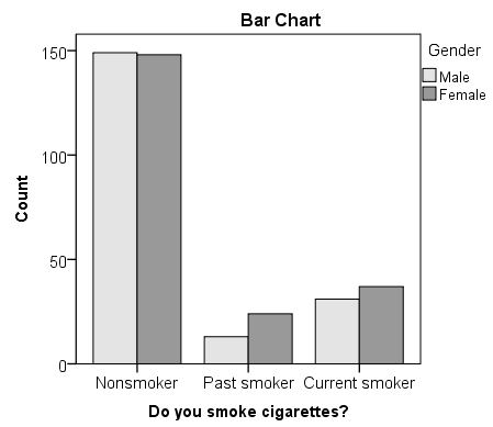
The "clusters" in a clustered bar chart are determined by the row variable (in this case, the smoking categories). The color of the bars is determined by the column variable (in this case, gender). The height of each bar represents the total number of observations in that particular combination of categories.

This type of chart emphasizes the differences within the categories of the row variable. Notice how within each smoking category, the heights of the bars (i.e., the number of males and females) are very similar. That is, there are an approximately equal number of male and female nonsmokers; approximately equal number of male and female past smokers; approximately equal number of male and female current smokers. If there were an association between gender and smoking, we would expect these counts to differ between groups in some way.

Running the Test

• Open the Crosstabs dialog ( Analyze > Descriptive Statistics > Crosstabs ).
• Select Smoking as the row variable, and Gender as the column variable.
• Click Statistics . Check Chi-square , then click Continue .
• (Optional) Check the box for Display clustered bar charts .

The first table is the Case Processing summary, which tells us the number of valid cases used for analysis. Only cases with nonmissing values for both smoking behavior and gender can be used in the test.

The next tables are the crosstabulation and chi-square test results.

The key result in the Chi-Square Tests table is the Pearson Chi-Square.

• The value of the test statistic is 3.171.
• The footnote for this statistic pertains to the expected cell count assumption (i.e., expected cell counts are all greater than 5): no cells had an expected count less than 5, so this assumption was met.
• Because the test statistic is based on a 3x2 crosstabulation table, the degrees of freedom (df) for the test statistic is $$ df = (R - 1)*(C - 1) = (3 - 1)*(2 - 1) = 2*1 = 2 $$.
• The corresponding p-value of the test statistic is p = 0.205.

Decision and Conclusions

Since the p-value is greater than our chosen significance level ( α = 0.05), we do not reject the null hypothesis. Rather, we conclude that there is not enough evidence to suggest an association between gender and smoking.

Based on the results, we can state the following:

• No association was found between gender and smoking behavior ( Χ 2 (2)> = 3.171, p = 0.205).

Example: Chi-square Test for 2x2 Table

Let's continue the row and column percentage example from the Crosstabs tutorial, which described the relationship between the variables RankUpperUnder (upperclassman/underclassman) and LivesOnCampus (lives on campus/lives off-campus). Recall that the column percentages of the crosstab appeared to indicate that upperclassmen were less likely than underclassmen to live on campus:

• The proportion of underclassmen who live off campus is 34.8%, or 79/227.
• The proportion of underclassmen who live on campus is 65.2%, or 148/227.
• The proportion of upperclassmen who live off campus is 94.4%, or 152/161.
• The proportion of upperclassmen who live on campus is 5.6%, or 9/161.

Suppose that we want to test the association between class rank and living on campus using a Chi-Square Test of Independence (using α = 0.05).

The clustered bar chart from the Crosstabs procedure can act as a complement to the column percentages above. Let's look at the chart produced by the Crosstabs procedure for this example:

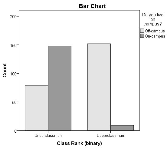
The height of each bar represents the total number of observations in that particular combination of categories. The "clusters" are formed by the row variable (in this case, class rank). This type of chart emphasizes the differences within the underclassmen and upperclassmen groups. Here, the differences in number of students living on campus versus living off-campus is much starker within the class rank groups.

• Select RankUpperUnder as the row variable, and LiveOnCampus as the column variable.
• (Optional) Click Cells . Under Counts, check the boxes for Observed and Expected , and under Residuals, click Unstandardized . Then click Continue .

The first table is the Case Processing summary, which tells us the number of valid cases used for analysis. Only cases with nonmissing values for both class rank and living on campus can be used in the test.

The next table is the crosstabulation. If you elected to check off the boxes for Observed Count, Expected Count, and Unstandardized Residuals, you should see the following table:

With the Expected Count values shown, we can confirm that all cells have an expected value greater than 5.

These numbers can be plugged into the chi-square test statistic formula:

$$ \chi^{2} = \sum_{i=1}^{R}{\sum_{j=1}^{C}{\frac{(o_{ij} - e_{ij})^{2}}{e_{ij}}}} = \frac{(-56.147)^{2}}{135.147} + \frac{(56.147)^{2}}{91.853} + \frac{(56.147)^{2}}{95.853} + \frac{(-56.147)^{2}}{65.147} = 138.926 $$

We can confirm this computation with the results in the Chi-Square Tests table:

The row of interest here is Pearson Chi-Square and its footnote.

• The value of the test statistic is 138.926.
• Because the crosstabulation is a 2x2 table, the degrees of freedom (df) for the test statistic is $$ df = (R - 1)*(C - 1) = (2 - 1)*(2 - 1) = 1 $$.
• The corresponding p-value of the test statistic is so small that it is cut off from display. Instead of writing "p = 0.000", we instead write the mathematically correct statement p < 0.001.

Since the p-value is less than our chosen significance level α = 0.05, we can reject the null hypothesis, and conclude that there is an association between class rank and whether or not students live on-campus.

• There was a significant association between class rank and living on campus ( Χ 2 (1) = 138.9, p < .001).
• << Previous: Analyzing Data
• Next: Pearson Correlation >>
• Last Updated: May 10, 2024 1:32 PM
• URL: https://libguides.library.kent.edu/SPSS

Street Address

Mailing address, quick links.

• How Are We Doing?
• Student Jobs

Information

• Accessibility
• Emergency Information
• For Our Alumni
• For the Media
• Jobs & Employment
• Life at KSU
• Privacy Statement
• Technology Support
• Website Feedback

Tutorial Playlist

Statistics tutorial, everything you need to know about the probability density function in statistics, the best guide to understand central limit theorem, an in-depth guide to measures of central tendency : mean, median and mode, the ultimate guide to understand conditional probability, a comprehensive look at percentile in statistics, the best guide to understand bayes theorem, everything you need to know about the normal distribution, an in-depth explanation of cumulative distribution function, a complete guide to chi-square test.

A Complete Guide on Hypothesis Testing in Statistics

Understanding the Fundamentals of Arithmetic and Geometric Progression

The definitive guide to understand spearman’s rank correlation, a comprehensive guide to understand mean squared error, all you need to know about the empirical rule in statistics, the complete guide to skewness and kurtosis, a holistic look at bernoulli distribution, all you need to know about bias in statistics, a complete guide to get a grasp of time series analysis.

The Key Differences Between Z-Test Vs. T-Test

The Complete Guide to Understand Pearson's Correlation

A complete guide on the types of statistical studies, everything you need to know about poisson distribution, your best guide to understand correlation vs. regression, the most comprehensive guide for beginners on what is correlation, what is a chi-square test formula, examples & application.

Lesson 9 of 24 By Avijeet Biswal

Table of Contents

The world is constantly curious about the Chi-Square test's application in machine learning and how it makes a difference. Feature selection is a critical topic in machine learning , as you will have multiple features in line and must choose the best ones to build the model. By examining the relationship between the elements, the chi-square test aids in the solution of feature selection problems. In this tutorial, you will learn about the chi-square test and its application.

What Is a Chi-Square Test?

The Chi-Square test is a statistical procedure for determining the difference between observed and expected data. This test can also be used to determine whether it correlates to the categorical variables in our data. It helps to find out whether a difference between two categorical variables is due to chance or a relationship between them.

Chi-Square Test Definition

A chi-square test is a statistical test that is used to compare observed and expected results. The goal of this test is to identify whether a disparity between actual and predicted data is due to chance or to a link between the variables under consideration. As a result, the chi-square test is an ideal choice for aiding in our understanding and interpretation of the connection between our two categorical variables.

A chi-square test or comparable nonparametric test is required to test a hypothesis regarding the distribution of a categorical variable. Categorical variables, which indicate categories such as animals or countries, can be nominal or ordinal. They cannot have a normal distribution since they can only have a few particular values.

For example, a meal delivery firm in India wants to investigate the link between gender, geography, and people's food preferences.

It is used to calculate the difference between two categorical variables, which are:

• As a result of chance or
• Because of the relationship

Your Data Analytics Career is Around The Corner!

Formula For Chi-Square Test

c = Degrees of freedom

O = Observed Value

E = Expected Value

The degrees of freedom in a statistical calculation represent the number of variables that can vary in a calculation. The degrees of freedom can be calculated to ensure that chi-square tests are statistically valid. These tests are frequently used to compare observed data with data that would be expected to be obtained if a particular hypothesis were true.

The Observed values are those you gather yourselves.

The expected values are the frequencies expected, based on the null hypothesis. 

Fundamentals of Hypothesis Testing

Hypothesis testing is a technique for interpreting and drawing inferences about a population based on sample data. It aids in determining which sample data best support mutually exclusive population claims.

Null Hypothesis (H0) - The Null Hypothesis is the assumption that the event will not occur. A null hypothesis has no bearing on the study's outcome unless it is rejected.

H0 is the symbol for it, and it is pronounced H-naught.

Alternate Hypothesis(H1 or Ha) - The Alternate Hypothesis is the logical opposite of the null hypothesis. The acceptance of the alternative hypothesis follows the rejection of the null hypothesis. H1 is the symbol for it.

Become a Data Science Expert & Get Your Dream Job

What Are Categorical Variables?

Categorical variables belong to a subset of variables that can be divided into discrete categories. Names or labels are the most common categories. These variables are also known as qualitative variables because they depict the variable's quality or characteristics.

Categorical variables can be divided into two categories:

• Nominal Variable: A nominal variable's categories have no natural ordering. Example: Gender, Blood groups
• Ordinal Variable: A variable that allows the categories to be sorted is ordinal variables. Customer satisfaction (Excellent, Very Good, Good, Average, Bad, and so on) is an example.

Why Do You Use the Chi-Square Test?

Chi-square is a statistical test that examines the differences between categorical variables from a random sample in order to determine whether the expected and observed results are well-fitting.

Here are some of the uses of the Chi-Squared test:

• The Chi-squared test can be used to see if your data follows a well-known theoretical probability distribution like the Normal or Poisson distribution.
• The Chi-squared test allows you to assess your trained regression model's goodness of fit on the training, validation, and test data sets.

Become an Expert in Data Analytics!

What Does A Chi-Square Statistic Test Tell You?

A Chi-Square test ( symbolically represented as  2 ) is fundamentally a data analysis based on the observations of a random set of variables. It computes how a model equates to actual observed data. A Chi-Square statistic test is calculated based on the data, which must be raw, random, drawn from independent variables, drawn from a wide-ranging sample and mutually exclusive. In simple terms, two sets of statistical data are compared -for instance, the results of tossing a fair coin. Karl Pearson introduced this test in 1900 for categorical data analysis and distribution. This test is also known as ‘Pearson’s Chi-Squared Test’. 

Chi-Squared Tests are most commonly used in hypothesis testing. A hypothesis is an assumption that any given condition might be true, which can be tested afterwards. The Chi-Square test estimates the size of inconsistency between the expected results and the actual results when the size of the sample and the number of variables in the relationship is mentioned. 

These tests use degrees of freedom to determine if a particular null hypothesis can be rejected based on the total number of observations made in the experiments. Larger the sample size, more reliable is the result.

There are two main types of Chi-Square tests namely -

Independence 

• Goodness-of-Fit 

The Chi-Square Test of Independence is a derivable ( also known as inferential ) statistical test which examines whether the two sets of variables are likely to be related with each other or not. This test is used when we have counts of values for two nominal or categorical variables and is considered as non-parametric test. A relatively large sample size and independence of obseravations are the required criteria for conducting this test.

For Example- 

In a movie theatre, suppose we made a list of movie genres. Let us consider this as the first variable. The second variable is whether or not the people who came to watch those genres of movies have bought snacks at the theatre. Here the null hypothesis is that th genre of the film and whether people bought snacks or not are unrelatable. If this is true, the movie genres don’t impact snack sales. 

Future-Proof Your AI/ML Career: Top Dos and Don'ts

Goodness-Of-Fit

In statistical hypothesis testing, the Chi-Square Goodness-of-Fit test determines whether a variable is likely to come from a given distribution or not. We must have a set of data values and the idea of the distribution of this data. We can use this test when we have value counts for categorical variables. This test demonstrates a way of deciding if the data values have a “ good enough” fit for our idea or if it is a representative sample data of the entire population. 

Suppose we have bags of balls with five different colours in each bag. The given condition is that the bag should contain an equal number of balls of each colour. The idea we would like to test here is that the proportions of the five colours of balls in each bag must be exact. 

Who Uses Chi-Square Analysis?

Chi-square is most commonly used by researchers who are studying survey response data because it applies to categorical variables. Demography, consumer and marketing research, political science, and economics are all examples of this type of research.

Let's say you want to know if gender has anything to do with political party preference. You poll 440 voters in a simple random sample to find out which political party they prefer. The results of the survey are shown in the table below:

To see if gender is linked to political party preference, perform a Chi-Square test of independence using the steps below.

Step 1: Define the Hypothesis

H0: There is no link between gender and political party preference.

H1: There is a link between gender and political party preference.

Step 2: Calculate the Expected Values

Now you will calculate the expected frequency.

For example, the expected value for Male Republicans is: 

Similarly, you can calculate the expected value for each of the cells.

Step 3: Calculate (O-E)2 / E for Each Cell in the Table

Now you will calculate the (O - E)2 / E for each cell in the table.

Step 4: Calculate the Test Statistic X2

X2  is the sum of all the values in the last table

 =  0.743 + 2.05 + 2.33 + 3.33 + 0.384 + 1

Before you can conclude, you must first determine the critical statistic, which requires determining our degrees of freedom. The degrees of freedom in this case are equal to the table's number of columns minus one multiplied by the table's number of rows minus one, or (r-1) (c-1). We have (3-1)(2-1) = 2.

Finally, you compare our obtained statistic to the critical statistic found in the chi-square table. As you can see, for an alpha level of 0.05 and two degrees of freedom, the critical statistic is 5.991, which is less than our obtained statistic of 9.83. You can reject our null hypothesis because the critical statistic is higher than your obtained statistic.

This means you have sufficient evidence to say that there is an association between gender and political party preference.

When to Use a Chi-Square Test?

A Chi-Square Test is used to examine whether the observed results are in order with the expected values. When the data to be analysed is from a random sample, and when the variable is the question is a categorical variable, then Chi-Square proves the most appropriate test for the same. A categorical variable consists of selections such as breeds of dogs, types of cars, genres of movies, educational attainment, male v/s female etc. Survey responses and questionnaires are the primary sources of these types of data. The Chi-square test is most commonly used for analysing this kind of data. This type of analysis is helpful for researchers who are studying survey response data. The research can range from customer and marketing research to political sciences and economics. 

The Ultimate Ticket to Top Data Science Job Roles

Chi-Square Distribution 

Chi-square distributions (X2) are a type of continuous probability distribution. They're commonly utilized in hypothesis testing, such as the chi-square goodness of fit and independence tests. The parameter k, which represents the degrees of freedom, determines the shape of a chi-square distribution.

A chi-square distribution is followed by very few real-world observations. The objective of chi-square distributions is to test hypotheses, not to describe real-world distributions. In contrast, most other commonly used distributions, such as normal and Poisson distributions, may explain important things like baby birth weights or illness cases per year.

Because of its close resemblance to the conventional normal distribution, chi-square distributions are excellent for hypothesis testing. Many essential statistical tests rely on the conventional normal distribution.

In statistical analysis , the Chi-Square distribution is used in many hypothesis tests and is determined by the parameter k degree of freedoms. It belongs to the family of continuous probability distributions . The Sum of the squares of the k independent standard random variables is called the Chi-Squared distribution. Pearson’s Chi-Square Test formula is - 

Where X^2 is the Chi-Square test symbol

Σ is the summation of observations

O is the observed results

E is the expected results 

The shape of the distribution graph changes with the increase in the value of k, i.e. degree of freedoms. 

When k is 1 or 2, the Chi-square distribution curve is shaped like a backwards ‘J’. It means there is a high chance that X^2 becomes close to zero. 

Courtesy: Scribbr

When k is greater than 2, the shape of the distribution curve looks like a hump and has a low probability that X^2 is very near to 0 or very far from 0. The distribution occurs much longer on the right-hand side and shorter on the left-hand side. The probable value of X^2 is (X^2 - 2).

When k is greater than ninety, a normal distribution is seen, approximating the Chi-square distribution.

Become a Data Scientist With Real-World Experience

Chi-Square P-Values

Here P denotes the probability; hence for the calculation of p-values, the Chi-Square test comes into the picture. The different p-values indicate different types of hypothesis interpretations. 

• P <= 0.05 (Hypothesis interpretations are rejected)
• P>= 0.05 (Hypothesis interpretations are accepted) 

The concepts of probability and statistics are entangled with Chi-Square Test. Probability is the estimation of something that is most likely to happen. Simply put, it is the possibility of an event or outcome of the sample. Probability can understandably represent bulky or complicated data. And statistics involves collecting and organising, analysing, interpreting and presenting the data. 

Finding P-Value

When you run all of the Chi-square tests, you'll get a test statistic called X2. You have two options for determining whether this test statistic is statistically significant at some alpha level:

• Compare the test statistic X2 to a critical value from the Chi-square distribution table.
• Compare the p-value of the test statistic X2 to a chosen alpha level.

Test statistics are calculated by taking into account the sampling distribution of the test statistic under the null hypothesis, the sample data, and the approach which is chosen for performing the test. 

The p-value will be as mentioned in the following cases.

• A lower-tailed test is specified by: P(TS ts | H0 is true) p-value = cdf (ts)
• Lower-tailed tests have the following definition: P(TS ts | H0 is true) p-value = cdf (ts)
• A two-sided test is defined as follows, if we assume that the test static distribution  of H0 is symmetric about 0. 2 * P(TS |ts| | H0 is true) = 2 * (1 - cdf(|ts|))

P: probability Event

TS: Test statistic is computed observed value of the test statistic from your sample cdf(): Cumulative distribution function of the test statistic's distribution (TS)

Types of Chi-square Tests

Pearson's chi-square tests are classified into two types:

• Chi-square goodness-of-fit analysis
• Chi-square independence test

These are, mathematically, the same exam. However, because they are utilized for distinct goals, we generally conceive of them as separate tests.

The chi-square test has the following significant properties:

• If you multiply the number of degrees of freedom by two, you will receive an answer that is equal to the variance.
• The chi-square distribution curve approaches the data is normally distributed as the degree of freedom increases.
• The mean distribution is equal to the number of degrees of freedom.

Properties of Chi-Square Test 

• Variance is double the times the number of degrees of freedom.
• Mean distribution is equal to the number of degrees of freedom.
• When the degree of freedom increases, the Chi-Square distribution curve becomes normal.

Limitations of Chi-Square Test

There are two limitations to using the chi-square test that you should be aware of. 

• The chi-square test, for starters, is extremely sensitive to sample size. Even insignificant relationships can appear statistically significant when a large enough sample is used. Keep in mind that "statistically significant" does not always imply "meaningful" when using the chi-square test.
• Be mindful that the chi-square can only determine whether two variables are related. It does not necessarily follow that one variable has a causal relationship with the other. It would require a more detailed analysis to establish causality.

Get In-Demand Skills to Launch Your Data Career

Chi-Square Goodness of Fit Test

When there is only one categorical variable, the chi-square goodness of fit test can be used. The frequency distribution of the categorical variable is evaluated for determining whether it differs significantly from what you expected. The idea is that the categories will have equal proportions, however, this is not always the case.

When you want to see if there is a link between two categorical variables, you perform the chi-square test. To acquire the test statistic and its related p-value in SPSS, use the chisq option on the statistics subcommand of the crosstabs command. Remember that the chi-square test implies that each cell's anticipated value is five or greater.

In this tutorial titled ‘The Complete Guide to Chi-square test’, you explored the concept of Chi-square distribution and how to find the related values. You also take a look at how the critical value and chi-square value is related to each other.

If you want to gain more insight and get a work-ready understanding in statistical concepts and learn how to use them to get into a career in Data Analytics , our Post Graduate Program in Data Analytics in partnership with Purdue University should be your next stop. A comprehensive program with training from top practitioners and in collaboration with IBM, this will be all that you need to kickstart your career in the field. 

Was this tutorial on the Chi-square test useful to you? Do you have any doubts or questions for us? Mention them in this article's comments section, and we'll have our experts answer them for you at the earliest!

1) What is the chi-square test used for? 

The chi-square test is a statistical method used to determine if there is a significant association between two categorical variables. It helps researchers understand whether the observed distribution of data differs from the expected distribution, allowing them to assess whether any relationship exists between the variables being studied.

2) What is the chi-square test and its types? 

The chi-square test is a statistical test used to analyze categorical data and assess the independence or association between variables. There are two main types of chi-square tests: a) Chi-square test of independence: This test determines whether there is a significant association between two categorical variables. b) Chi-square goodness-of-fit test: This test compares the observed data to the expected data to assess how well the observed data fit the expected distribution.

3) What is the chi-square test easily explained? 

The chi-square test is a statistical tool used to check if two categorical variables are related or independent. It helps us understand if the observed data differs significantly from the expected data. By comparing the two datasets, we can draw conclusions about whether the variables have a meaningful association.

4) What is the difference between t-test and chi-square? 

The t-test and the chi-square test are two different statistical tests used for different types of data. The t-test is used to compare the means of two groups and is suitable for continuous numerical data. On the other hand, the chi-square test is used to examine the association between two categorical variables. It is applicable to discrete, categorical data. So, the choice between the t-test and chi-square test depends on the nature of the data being analyzed.

5) What are the characteristics of chi-square? 

The chi-square test has several key characteristics:

1) It is non-parametric, meaning it does not assume a specific probability distribution for the data.

2) It is sensitive to sample size; larger samples can result in more significant outcomes.

3) It works with categorical data and is used for hypothesis testing and analyzing associations.

4) The test output provides a p-value, which indicates the level of significance for the observed relationship between variables.

5)It can be used with different levels of significance (e.g., 0.05 or 0.01) to determine statistical significance.

Find our Data Analyst Online Bootcamp in top cities:

About the author.

Avijeet is a Senior Research Analyst at Simplilearn. Passionate about Data Analytics, Machine Learning, and Deep Learning, Avijeet is also interested in politics, cricket, and football.

Recommended Resources

Getting Started with Google Display Network: The Ultimate Beginner’s Guide

Sanity Testing Vs Smoke Testing: Know the Differences, Applications, and Benefits Of Each

Fundamentals of Software Testing

The Building Blocks of API Development

• PMP, PMI, PMBOK, CAPM, PgMP, PfMP, ACP, PBA, RMP, SP, and OPM3 are registered marks of the Project Management Institute, Inc.

• Math Article
• Chi Square Test

Chi-Square Test

A chi-squared test  (symbolically represented as  χ 2 ) is basically a data analysis on the basis of observations of a random set of variables. Usually, it is a comparison of two statistical data sets. This test was introduced by Karl Pearson in 1900 for categorical data analysis and distribution . So it was mentioned as Pearson’s chi-squared test .

The chi-square test is used to estimate how likely the observations that are made would be, by considering the assumption of the null hypothesis as true.

A hypothesis is a consideration that a given condition or statement might be true, which we can test afterwards. Chi-squared tests are usually created from a sum of squared falsities or errors over  the sample variance.

Chi-Square Distribution

When we consider, the null speculation is true, the sampling distribution of the test statistic is called as chi-squared distribution . The chi-squared test helps to determine whether there is a notable difference between the normal frequencies and the observed frequencies in one or more classes or categories. It gives the probability of independent variables.

Note: Chi-squared test is applicable only for categorical data, such as men and women falling under the categories of Gender, Age, Height, etc.

Finding P-Value

P stands for probability here. To calculate the p-value, the chi-square test is used in statistics. The different values of p indicates the different hypothesis interpretation, are given below:

• P≤ 0.05; Hypothesis rejected
• P>.05; Hypothesis Accepted

Probability is all about chance or risk or uncertainty. It is the possibility of the outcome of the sample or the occurrence of an event. But when we talk about statistics, it is more about how we handle various data using different techniques. It helps to represent complicated data or bulk data in a very easy and understandable way. It describes the collection, analysis, interpretation, presentation, and organization of data. The concept of both probability and statistics is related to the chi-squared test.

Also, read:

The following are the important properties of the chi-square test:

• Two times the number of degrees of freedom is equal to the variance.
• The number of degree of freedom is equal to the mean distribution
• The chi-square distribution curve approaches the normal distribution when the degree of freedom increases.

The chi-squared test is done to check if there is any difference between the observed value and expected value. The formula for chi-square can be written as;

χ 2  = ∑(O i – E i ) 2 /E i

where O i is the observed value and E i is the expected value.

Chi-Square Test of Independence

The chi-square test of independence also known as the chi-square test of association which is used to determine the association between the categorical variables. It is considered as a non-parametric test . It is mostly used to test statistical independence.

The chi-square test of independence is not appropriate when the categorical variables represent the pre-test and post-test observations. For this test, the data must meet the following requirements:

• Two categorical variables
• Relatively large sample size
• Categories of variables (two or more)
• Independence of observations

Example of Categorical Data

Let us take an example of a categorical data where there is a society of 1000 residents with four neighbourhoods, P, Q, R and S. A random sample of 650 residents of the society is taken whose occupations are doctors, engineers and teachers. The null hypothesis is that each person’s neighbourhood of residency is independent of the person’s professional division. The data are categorised as:

Assume the sample living in neighbourhood P, 150, to estimate what proportion of the whole 1,000 people live in neighbourhood P. In the same way, we take 349/650 to calculate what ratio of the 1,000 are doctors. By the supposition of independence under the hypothesis, we should “expect” the number of doctors in neighbourhood P is;

150 x 349/650  ≈ 80.54

So by  the chi-square test formula for that particular cell in the table, we get;

(Observed – Expected) 2 /Expected Value = (90-80.54) 2 /80.54  ≈ 1.11

Some of the exciting facts about the Chi-square test are given below:

The Chi-square statistic can only be used on numbers. We cannot use them for data in terms of percentages, proportions, means or similar statistical contents. Suppose, if we have 20% of 400 people, we need to convert it to a number, i.e. 80, before running a test statistic.

A chi-square test will give us a p-value. The p-value will tell us whether our test results are significant or not. 

However, to perform a chi-square test and get the p-value, we require two pieces of information:

(1) Degrees of freedom. That’s just the number of categories minus 1.

(2) The alpha level(α). You or the researcher chooses this. The usual alpha level is 0.05 (5%), but you could also have other levels like 0.01 or 0.10.

In elementary statistics, we usually get questions along with the degrees of freedom(DF) and the alpha level. Thus, we don’t usually have to figure out what they are. To get the degrees of freedom, count the categories and subtract 1.

The chi-square distribution table with three probability levels is provided here. The statistic here is used to examine whether distributions of certain variables vary from one another. The categorical variable will produce data in the categories and numerical variables will produce data in numerical form.

The distribution of χ 2 with (r-1)(c-1) degrees of freedom(DF) , is represented in the table given below. Here, r represents the number of rows in the two-way table and c represents the number of columns.

Solved Problem

 A survey on cars had conducted in 2011 and determined that 60% of car owners have  only one car, 28% have two cars, and 12% have three or more. Supposing that you have decided to conduct your own survey and have collected the data below, determine whether your data supports the results of the study.

Use a significance level of 0.05. Also, given that, out of 129 car owners, 73 had one car and 38 had two cars.

Let us state the null and alternative hypotheses.

H 0 : The proportion of car owners with one, two or three cars is 0.60, 0.28 and 0.12 respectively.

H 1 : The proportion of car owners with one, two or three cars does not match the proposed model.

A Chi-Square goodness of fit test is appropriate because we are examining the distribution of a single categorical variable. 

Let’s tabulate the given information and calculate the required values.

Therefore, χ 2  = ∑(O i  – E i ) 2 /E i  = 0.7533

Let’s compare it to the chi-square value for the significance level 0.05. 

The degrees for freedom = 3 – 1 = 2

Using the table, the critical value for a 0.05 significance level with df = 2 is 5.99. 

That means that 95 times out of 100, a survey that agrees with a sample will have a χ 2  value of 5.99 or less. 

The Chi-square statistic is only 0.7533, so we will accept the null hypothesis.

Frequently Asked Questions – FAQs

What is the chi-square test write its formula, how do you calculate chi squared, what is a chi-square test used for, how do you interpret a chi-square test, what is a good chi-square value, leave a comment cancel reply.

Your Mobile number and Email id will not be published. Required fields are marked *

Request OTP on Voice Call

Post My Comment

Register with BYJU'S & Download Free PDFs

Register with byju's & watch live videos.

Statistics Made Easy

5 Tips for Choosing the Right Statistical Test

One of the most important and potentially challenging parts of statistical analysis is ensuring that the statistical test used aligns with the research question and available data. Common statistical tests include t-tests, Chi-squared, ANOVA, regression analysis, and more, and each is suited to different types of data and research questions. Using the wrong statistical test can lead to misleading conclusions, compromised data integrity, and invalid results. It can result in either Type I errors, where you incorrectly reject a true null hypothesis, or Type II errors, where you fail to detect a true effect. By carefully considering factors such as the nature of your data, your research question, and the assumptions underlying each test, you can ensure that your statistical analysis is robust and reliable. This article provides five essential tips to guide you in selecting the right statistical test for your research.

1. Understand Your Data

The foundation of any statistical analysis begins with a thorough understanding of the available data. First, it is important to recognize the types of data available. Categorical data, for example, includes variables that can be grouped into categories but have no inherent order, such as preferred color. Ordinal data, on the other hand, has categories in a clear order, but no consistent difference between those categories, such as levels of satisfaction. Interval and ratio data are both numeric with interval data lacking a true zero and ratio data having a meaningful zero point.

Besides the type of data, understanding the available data also includes knowing the distribution and variability. Visualizations like bar graphs and scatterplots can be utilized based on the variable types. Descriptive statistics of central tendency and variability can also describe the main features of the dataset. Finally, verifying whether numerical data is normally distributed can be essential for certain types of statistical tests. 

2. Develop a Research Question

Before selecting and running any statistical test, a research question must be in place to guide the analysis. This involves identifying the primary aim of the sturdy and specifying what exactly you seek to uncover from the data. A good research question will be highly specific and testable. For example, “what impacts customer satisfaction with the notebook” is not a good research question upon which to build a statistical test as it is too vague. On the other hand, “what notebook color do customers prefer” is specific and testable as satisfaction scores for different colored notebooks can be specifically compared. 

3. Consider the Comparison You are Making

Once you have a specific and testable research question, consider what type of comparison that research question is making. Different statistical tests can make different types of comparisons based on what types of variables are present and what comparison is being made.

One class of statistical tests, including t-tests and ANOVAs, can compare a numerical variables between two or more groups. For example, an ANOVA can test if the mean satisfaction score is different between red, blue, and green notebooks to see if there is a statistically significant difference. 

Another class can compare two numerical variables with each other. In these cases, correlation and regression analyses are commonly used. Correlations measure the strength and direction of the relationship between two variables while regressions go a step further and model the relationship, allowing for predictions to be made based on the data. 

Finally, there are tests that can compare two categorical variables and determine if there is an association, such as the relationship between gender and preferred color. 

4. Consult Statistical References

Once all of these factors impacting the selection of a statistical test are understood, a statistical reference can be consulted to finalize the test decision. The most commonly used references are flow charts that start by asking what type of data is being compared, numerical or categorical. Then, you select the type of comparison you are running. Additional questions and branches of the flow chart ultimately lead you to a statistical test that matches the analysis you are running. 

One such flow chart is available from Colorado State University. Taking the example research question “what notebook color do customers prefer”, and assuming that the preference score is continuous and normally distributed and that you are comparing more than two colors, this would lead to selecting an ANOVA test.

5. Check the Assumptions of Your Test

Finally, before carrying out the statistical test, it is essential to verify that the data meets the assumptions required by that test. Some of these assumptions, such as requiring continuous data across more than two categories for an ANOVA analysis, have already been validated by this point. However, each test will also have its own set of assumptions that need to be verified to ensure that the conclusions are correct and reliable. 

For example, many tests require that the continuous variables be normally distributed and that all the variables included be independent from each other. Most tests also require all the data points to be independent of each other, so including the same person more than once is usually not permitted.

If the assumptions of a statistical test are not met, alternative methods like non-parametric tests can be considered. Alternatively, the existing data can be transformed, more data can be collected, or outliers can be removed where justified.

Choosing the right statistical test is a pivotal aspect of conducting robust and reliable research. By understanding your data, developing a clear research question, considering the comparisons you are making, performing exploratory data analysis, and checking the assumptions of your chosen test, you can significantly enhance the accuracy and credibility of your findings. When assumptions are not met, adapting your approach through data transformation, non-parametric tests, or other robust methods ensures the integrity of your analysis. With these five essential, you are well-equipped to make informed decisions in your statistical testing, leading to more meaningful and valid conclusions.

Featured Posts

Leave a Reply Cancel reply

Your email address will not be published. Required fields are marked *

Join the Statology Community

Sign up to receive Statology's exclusive study resource: 100 practice problems with step-by-step solutions. Plus, get our latest insights, tutorials, and data analysis tips straight to your inbox!

By subscribing you accept Statology's Privacy Policy.

Thank you for visiting nature.com. You are using a browser version with limited support for CSS. To obtain the best experience, we recommend you use a more up to date browser (or turn off compatibility mode in Internet Explorer). In the meantime, to ensure continued support, we are displaying the site without styles and JavaScript.

• View all journals
• My Account Login
• Explore content
• About the journal
• Publish with us
• Sign up for alerts
• Registered Report
• Open access
• Published: 27 May 2024

Comparing researchers’ degree of dichotomous thinking using frequentist versus Bayesian null hypothesis testing

• Jasmine Muradchanian   ORCID: orcid.org/0000-0002-2914-9197 1 ,
• Rink Hoekstra 1 ,
• Henk Kiers 1 ,
• Dustin Fife 2 &
• Don van Ravenzwaaij 1  

Scientific Reports volume  14 , Article number:  12120 ( 2024 ) Cite this article

31 Accesses

Metrics details

• Human behaviour
• Neuroscience

A large amount of scientific literature in social and behavioural sciences bases their conclusions on one or more hypothesis tests. As such, it is important to obtain more knowledge about how researchers in social and behavioural sciences interpret quantities that result from hypothesis test metrics, such as p -values and Bayes factors. In the present study, we explored the relationship between obtained statistical evidence and the degree of belief or confidence that there is a positive effect in the population of interest. In particular, we were interested in the existence of a so-called cliff effect: A qualitative drop in the degree of belief that there is a positive effect around certain threshold values of statistical evidence (e.g., at p  = 0.05). We compared this relationship for p -values to the relationship for corresponding degrees of evidence quantified through Bayes factors, and we examined whether this relationship was affected by two different modes of presentation (in one mode the functional form of the relationship across values was implicit to the participant, whereas in the other mode it was explicit). We found evidence for a higher proportion of cliff effects in p -value conditions than in BF conditions (N = 139), but we did not get a clear indication whether presentation mode had an effect on the proportion of cliff effects.

Protocol registration

The stage 1 protocol for this Registered Report was accepted in principle on 2 June 2023. The protocol, as accepted by the journal, can be found at: https://doi.org/10.17605/OSF.IO/5CW6P .

Similar content being viewed by others

Testing theory of mind in large language models and humans

Microdosing with psilocybin mushrooms: a double-blind placebo-controlled study

Determinants of behaviour and their efficacy as targets of behavioural change interventions

Introduction.

In applied science, researchers typically conduct statistical tests to learn whether an effect of interest differs from zero. Such tests typically tend to quantify evidence by means of p -values (but see e.g., Lakens 1 who warns against such an interpretation of p -values). A Bayesian alternative to the p -value is the Bayes factor (BF), which is a tool used for quantifying statistical evidence in hypothesis testing 2 , 3 . P -values and BFs are related to one another 4 , with BFs being used much less frequently. Having two contrasting hypotheses (i.e., a null hypothesis, H 0 , and an alternative hypothesis, H 1 ), a p -value is the probability of getting a result as extreme or more extreme than the actual observed sample result, given that H 0 were true (and given that the assumptions hold). A BF on the other hand, quantifies the probability of the data given H 1 relative to the probability of the data given H 0 (called BF 10 3 ).

There is ample evidence that researchers often find it difficult to interpret quantities such as p -values 5 , 6 , 7 . Although there has been growing awareness of the dangers of misinterpreting p -values, these dangers seem to remain prevalent. One of the key reasons for these misinterpretations is that these concepts are not simple or intuitive, and the correct interpretation of them would require more cognitive effort. Because of this high cognitive demand academics have been using shortcut interpretations, which are simply wrong 6 . An example of such a misinterpretation is that the p -value would represent the probability of the null hypothesis being true 6 . Research is typically conducted in order to reduce uncertainty around the existence of an effect in the population of interest. To do this, we use measures such as p -values and Bayes factors as a tool. Hence, it might be interesting (especially given the mistakes that are made by researchers when interpreting quantities such as p -values) to study how these measures affect people’s beliefs regarding the existence of an effect in the population of interest, so one can study how outcomes like p -values and Bayes factors translate to subjective beliefs about the existence of an effect in practice.

One of the first studies that focused on how researchers interpret statistical quantities was conducted by Rosenthal and Gaito 8 , in which they specifically studied how researchers interpret p -values of varying magnitude. Nineteen researchers and graduate students at their psychology faculty were requested to indicate their degree of belief or confidence in 14 p -values, varying from 0.001 to 0.90, on a 6-point scale ranging from “5 extreme confidence or belief” to “0 complete absence of confidence or belief” 8 , pp. 33–34 . These individuals were shown p -values for sample sizes of 10 and 100. The authors wanted to measure the degree of belief or confidence in research findings as a function of associated p -values, but stated as such it is not really clear what is meant here. We assume that the authors actually wanted to assess degree of belief or confidence in the existence of an effect, given the p -value. Their findings suggested that subjects’ degree of belief or confidence appeared to be a decreasing exponential function of the p- value. Additionally, for any p -value, self-rated confidence was greater for the larger sample size (i.e., n  = 100). Furthermore, the authors argued in favor of the existence of a cliff effect around p  = 0.05, which refers to an abrupt drop in the degree of belief or confidence in a p -value just beyond the 0.05 level 8 , 9 . This finding has been confirmed in several subsequent studies 10 , 11 , 12 . The studies described so far have been focusing on the average, and have not taken individual differences into account.

The cliff effect suggests p -values invite dichotomous thinking, which according to some authors seems to be a common type of reasoning when interpreting p -values in the context of Null Hypothesis Significance Testing (NHST 13 ). The outcome of the significance test seems to be usually interpreted dichotomously such as suggested by studies focusing on the cliff effect 8 , 9 , 10 , 11 , 12 , 13 , where one makes a binary choice between rejecting or not rejecting a null hypothesis 14 . This practice has taken some academics away from the main task of finding out the size of the effect of interest and the level of precision with which it has been measured 5 . However, Poitevineau and Lecoutre 15 argued that the cliff effect around p  = 0.05 is probably overstated. According to them, previous studies paid insufficient attention to individual differences. To demonstrate this, they explored the individual data and found qualitative heterogeneity in the respondents’ answers. The authors identified three categories of functions based on 12 p -values: (1) a decreasing exponential curve, (2) a decreasing linear curve, and (3) an all-or-none curve representing a very high degree of confidence when p  ≤ 0.05 and quasi-zero confidence otherwise. Out of 18 participants, they found that the responses of 10 participants followed a decreasing exponential curve, 4 participants followed a decreasing linear curve, and 4 participants followed an all-or-none curve. The authors concluded that the cliff effect may be an artifact of averaging, resulting from the fact that a few participants have an all-or-none interpretation of statistical significance 15 .

Although NHST has been used frequently, it has been argued that it should be replaced by effect sizes, confidence intervals (CIs), and meta-analyses. Doing so may allegedly invite a shift from dichotomous thinking to estimation and meta-analytic thinking 14 . Lai et al. 13 studied whether using CIs rather than p -values would reduce the cliff effect, and thereby dichotomous thinking. Similar to the classification by Poitevineau and Lecoutre 15 , the responses were divided into three classes: decreasing exponential, decreasing linear, or all-or-none. In addition, Lai et al. 13 found patterns in the responses of some of the participants that corresponded with what they called a “moderate cliff model”, which refers to using statistical significance as both a decision-making criterion and a measure of evidence 13 .

In contrast to Poitevineau and Lecoutre 15 , Lai et al. 13 concluded that the cliff effect is probably not just a byproduct resulting from the all-or-none class, because the cliff models were accountable for around 21% of the responses in NHST interpretation and for around 33% of the responses in CI interpretation. Furthermore, a notable finding was that the cliff effect prevalence in CI interpretations was more than 50% higher than that of NHST 13 . Something similar was found in a study by Hoekstra, Johnson, and Kiers 16 . They also predicted that the cliff effect would be stronger for results presented in the NHST format compared to the CI format, and like Lai et al. 13 , they actually found more evidence of a cliff effect in the CI format compared to the NHST format 16 .

The studies discussed so far seem to provide evidence for the existence of a cliff effect around p  = 0.05. Table 1 shows an overview of evidence related to the cliff effect. Interestingly, in a recent study, Helske et al. 17 examined how various visualizations can aim in reducing the cliff effect when interpreting inferential statistics among researchers. They found that compared to textual representation of the CI with p -values and classic CI visualization, including more complex visual information to classic CI representation seemed to decrease the cliff effect (i.e., dichotomous interpretations 17 ).

Although Bayesian methods have become more popular within different scientific fields 18 , 19 , we know of no studies that have examined whether self-reported degree of belief of the existence of an effect when interpreting BFs by researchers results in a similar cliff effect to those obtained for p -values and CIs. Another matter that seems to be conspicuously absent in previous examinations of the cliff effect is a comparison between the presentation methods that are used to investigate the cliff effect. In some cliff effect studies the p -values were presented to the participants on separate pages 15 and in other cliff effect studies the p -values were presented on the same page 13 . It is possible that the cliff effect manifests itself in (some) researchers without explicit awareness. It is possible that for those researchers presenting p -values/Bayes factors in isolation would lead to a cliff effect, whereas presenting all p -values/Bayes factors at once would lead to a cognitive override. Perhaps when participants see their cliff effect, they might think that they should not think dichotomously, and might change their results to be more in line with how they believe they should think, thereby removing their cliff effect. To our knowledge, no direct comparison of p -values/Bayes factors in isolation and all p -values/Bayes factors at once has yet been conducted. Therefore, to see whether the method matters, both types of presentation modes will be included in the present study.

All of this gives rise to the following three research questions: (1) What is the relation between obtained statistical evidence and the degree of belief or confidence that there is a positive effect in the population of interest across participants? (2) What is the difference in this relationship when the statistical evidence is quantified through p -values versus Bayes factors? (3) What is the difference in this relationship when the statistical evidence is presented in isolation versus all at once?

In the present study, we will investigate the relationship between method (i.e., p -values and Bayes factors) and the degree of belief or confidence that there is a positive effect in the population of interest, with special attention for the cliff effect. We choose this specific wording (“positive effect in the population of interest”) as we believe that this way of phrasing is more specific than those used in previous cliff effect studies. We will examine the relationship between different levels of strength of evidence using p -values or corresponding Bayes factors and measure participants' degree of belief or confidence in the following two scenarios: (1) the scenario in which values will be presented in isolation (such that the functional form of the relationship across values is implicit to the participant) and (2) the scenario in which all values will be presented simultaneously (such that the functional form of the relationship across values is explicit to the participant).

In what follows, we will first describe the set-up of the present study. In the results section, we will explore the relationship between obtained statistical evidence and the degree of belief or confidence, and in turn, we will compare this relationship for p -values to the corresponding relationship for BFs. All of this will be done in scenarios in which researchers are either made aware or not made aware of the functional form of the relationship. In the discussion, we will discuss implications for applied researchers using p -values and/or BFs in order to quantify statistical evidence.

Ethics information

Our study protocol has been approved by the ethics committee of the University of Groningen and our study complies with all relevant ethical regulations of the University of Groningen. Informed consent will be obtained from all participants. As an incentive for participating, we will raffle 10 Amazon vouchers with a worth of 25USD among participants that successfully completed our study.

Sampling plan

Our target population will consist of researchers in the social and behavioural sciences who are at least somewhat familiar with interpreting Bayes factors. We will obtain our prospective sample by collecting the e-mail addresses of (approximately) 2000 corresponding authors from 20 different journals in social and behavioural sciences with the highest impact factor. Specifically, we will collect the e-mail addresses of 100 researchers who published an article in the corresponding journal in 2021. We will start with the first issue and continue until we have 100 e-mail addresses per journal. We will contact the authors by e-mail. In the e-mail we will mention that we are looking for researchers who are familiar with interpreting Bayes factors. If they are familiar with interpreting Bayes factors, then we will ask them to participate in our study. If they are not familiar with interpreting Bayes factors, then we will ask them to ignore our e-mail.

If the currently unknown response rate is too low to answer our research questions, we will collect additional e-mail addresses of corresponding authors from articles published in 2022 in the same 20 journals. Based on a projected response rate of 10%, we expect a final completion rate of 200 participants. This should be enough to obtain a BF higher than 10 in favor of an effect if the proportions differ by 0.2 (see section “ Planned analyses ” for details).

Materials and procedure

The relationship between the different magnitudes of p -values/BFs and the degree of belief or confidence will be examined in a scenario in which values will be presented in isolation and in a scenario in which the values will be presented simultaneously. This all will result in four different conditions: (1) p -value questions in the isolation scenario (isolated p -value), (2) BF questions in the isolation scenario (isolated BF), (3) p -value questions in the simultaneous scenario (all at once p -value), and (4) BF questions in the simultaneous scenario (all at once BF). To reduce boredom, and to try to avoid making underlying goals of the study too apparent, each participant will receive randomly one out of four scenarios (i.e., all at once p -value, all at once BF, isolated p -value, or isolated BF), so the study has a between-person design.

The participants will receive an e-mail with an anonymous Qualtrics survey link. The first page of the survey will consist of the informed consent. We will ask all participants to indicate their level of familiarity with both Bayes factors and p -values on a 3-point scale with “completely unfamiliar/somewhat familiar/very familiar” and we will include everyone who is at least somewhat familiar on both. To have a better picture of our sample population, we will include the following demographic variables in the survey: gender, main continent, career stage, and broad research area. Then we will randomly assign respondents to one of four conditions (see below for a detailed description). After completing the content-part of the survey, all respondents will receive a question about providing their e-mail address if they are interested in (1) being included in the random draw of the Amazon vouchers; or (2) receiving information on our study outcomes.

In the isolated p -value condition, the following fabricated experimental scenario will be presented:

“Suppose you conduct an experiment comparing two independent groups, with n = 250 in each group. The null hypothesis states that the population means of the two groups do not differ. The alternative hypothesis states that the population mean in group 1 is larger than the population mean in group 2. Suppose a two-sample t test was conducted and a one-sided p value calculated.”

Then a set of possible findings of the fabricated experiment will be presented at different pages. We varied the strength of evidence for the existence of a positive effect with the following ten p -values in a random order: 0.001, 0.002, 0.004, 0.008, 0.016, 0.032, 0.065, 0.131, 0.267, and 0.543. A screenshot of a part of the isolated p -value questions is presented in S1 in the Supplementary Information.

In the all at once BF condition, a fabricated experimental scenario will be presented identical to that in the isolated p -value condition, except the last part is replaced by:

“Suppose a Bayesian two-sample t test was conducted and a one-sided Bayes factor (BF) calculated, with the alternative hypothesis in the numerator and the null hypothesis in the denominator, denoted BF 10 .”

A set of possible findings of the fabricated experiment will be presented at the same page. These findings vary in terms of the strength of evidence for the existence of a positive effect, quantified with the following ten BF 10 values in the following order: 22.650, 12.008, 6.410, 3.449, 1.873, 1.027, 0.569, 0.317, 0.175, and 0.091. These BF values correspond one-on-one to the p -values presented in the isolated p -value condition (the R code for the findings of the fabricated experiment can be found on https://osf.io/sq3fp ). A screenshot of a part of the all at once BF questions can be found in S2 in the Supplementary Information.

In both conditions, the respondents will be asked to rate their degree of belief or confidence that there is a positive effect in the population of interest based on these findings on a scale ranging from 0 (completely convinced that there is no effect), through 50 (somewhat convinced that there is a positive effect), to 100 (completely convinced that there is a positive effect).

The other two conditions (i.e., isolated BF condition and the all at once p -value condition) will be the same as the previously described conditions. The only difference between these two conditions and the previously described conditions is that in the isolated BF condition, the findings of the fabricated experiment for the BF questions will be presented at different pages in a random order, and in the all at once p -value condition, the findings for the p -value questions will be presented at the same page in a non-random order.

To keep things as simple as possible for the participants, all fictitious scenarios will include a two-sample t test with either a one-tailed p -value or a BF. The total sample size will be large ( n  = 250 in each group) in order to have sufficiently large power to detect even small effects.

Planned analyses

Poitevineau and Lecoutre 15 have suggested the following three models for the relationships between the different levels of statistical evidence and researchers’ subjective belief that a non-zero effect exists: all-or-none ( y  =  a for p  < 0.05, y  =  b for p  ≥ 0.05), linear ( y  =  a  +  bp ), and exponential ( y  = exp( a  +  bp )). In addition, Lai et al. 13 have suggested the moderate cliff model (a more gradual version of all-or-none), which they did not define more specifically. In the study by Lai et al. 13 (Fig.  4 ), the panel that represents the moderate cliff seems to be a combination of the exponential and the all-or-none function. In the present study, we will classify responses as moderate cliff if we observe a steep drop in the degree of belief or confidence around a certain p -value/BF, while for the remaining p -values/BFs the decline in confidence is more gradual. So, for example, a combination of the decreasing linear and the all-or-none function will also be classified as moderate cliff in the present study. Plots of the four models with examples of reasonable choices for the parameters are presented in Fig.  1 (the R code for Fig.  1 can be found on https://osf.io/j6d8c ).

Plots are shown for fictitious outcomes for the four models (all-or-none, linear, exponential, and moderate cliff). The x-axis represents the different p -values. In the two BF conditions, the x-axis represents the different BF values. The y-axis represents the proportion of degree of belief or confidence that there is a positive effect in the population of interest. Note that these are prototype responses; different variations on these response patterns are possible.

We will manually classify data for each participant for each scenario as one of the relationship models. We will do so by blinding the coders as to the conditions associated with the data. Specifically, author JM will organize the data from each of the four conditions and remove the p -value or BF labels. Subsequently, authors DvR and RH will classify the data independently from one another. In order to improve objectivity regarding the classification, authors DvR and RH will classify the data according to specific instructions that are constructed before collecting the data (see Appendix 1 ). After coding, we will compute Cohen’s kappa for these data. For each set of scores per condition per subject for which there was no agreement on classification, authors DvR and RH will try to reach consensus in a discussion of no longer than 5 min. If after this discussion no agreement is reached, then author DF will classify these data. If author DF will choose the same class as either DvR or RH, then the data will be classified accordingly. However, if author DF will choose another class, then the data will be classified in a so-called rest category. This rest category will also include data that extremely deviate from the four relationship models, and we will assess these data by running exploratory analyses. Before classifying the real data, we will conduct a small pilot study in order to provide authors DvR and RH with the possibility to practice classifying the data. In the Qualtrics survey, the respondents cannot continue with the next question without answering the current question. However, it might be possible that some of the respondents quit filling out the survey. The responses of the participants who did not answer all questions will be removed from the dataset. This means that we will use complete case analysis in order to deal with missing data, because we do not expect to find specific patterns in the missing values.

Our approach to answer Research Question 1 (RQ1; “What is the relation between obtained statistical evidence and the degree of belief or confidence that there is a positive effect in the population of interest across participants?”) will be descriptive in nature. We will explore the results visually, by assessing the four models (i.e., all-or-none, linear, exponential, and moderate cliff) in each of the four conditions (i.e., isolated p -value, all at once p -value, isolated BF, and all at once BF), followed by zooming in on the classification ‘cliff effect’. This means that we will compare the frequency of the four classification models with one another within each of the four conditions.

In order to answer Research Question 2 (RQ2; “What is the difference in this relationship when the statistical evidence is quantified through p -values versus Bayes factors?”), we will first combine categories as follows: the p -value condition will encompass the data from both the isolated and the all at once p -value conditions, and the BF condition will encompass the data from both the isolated and the all at once BF conditions. Furthermore, the cliff condition will encompass the all-or-none and the moderate cliff models, and the non-cliff condition will encompass the linear and the exponential models. This classification ensures that we distinguish between curves that reflect a sudden change in the relationship between the level of statistical evidence and the degree of confidence that a positive effect exists in the population of interest, and those that represent a gradual relationship between the level of statistical evidence and the degree of confidence. We will then compare the proportions of cases with a cliff in the p -value conditions to those in the BF conditions, and we will add inferential information for this comparison by means of a Bayesian chi square test on the 2 × 2 table ( p -value/BF x cliff/non-cliff), as will be specified below.

Finally, in order to answer Research Question 3 (RQ3; “What is the difference in this relationship when the statistical evidence is presented in isolation versus all at once?”), we will first combine categories again, as follows: the isolation condition will encompass the data from both the isolated p -value and the isolated BF conditions, and the all at once condition will encompass the data from both the all at once p -value and the all at once BF conditions. The cliff/non-cliff distinction is made analogous to the one employed for RQ2. We will then compare the proportions of cases with a cliff in the isolated conditions to those in the all at once conditions, and we will add inferential information for this comparison by means of a Bayesian chi square test on the 2 × 2 table (all at once/isolated x cliff/non-cliff), as will be specified below.

For both chi square tests, the null hypothesis states that there is no difference in the proportion of cliff classifications between the two conditions, and the alternative hypothesis states that there is a difference in the proportion of cliff classifications between the two conditions. Under the null hypothesis, we specify a single beta(1,1) prior for the proportion of cliff classifications and under the alternative hypothesis we specify two independent beta(1,1) priors for the proportion of cliff classifications 20 , 21 . A beta(1,1) prior is a flat or uniform prior from 0 to 1. The Bayes factor that will result from both chi square tests gives the relative evidence for the alternative hypothesis over the null hypothesis (BF 10 ) provided by the data. Both tests will be carried out in RStudio 22 (the R code for calculating the Bayes factors can be found on https://osf.io/5xbzt ). Additionally, the posterior of the difference in proportions will be provided (the R code for the posterior of the difference in proportions can be found on https://osf.io/3zhju ).

If, after having computed results on the obtained sample, we observe that our BFs are not higher than 10 or smaller than 0.1, we will expand our sample in the way explained at the end of section “Sampling Plan”. To see whether this approach will likely lead to useful results, we have conducted a Bayesian power simulation study for the case of population proportions of 0.2 and 0.4 (e.g., 20% cliff effect in the p -value group, and 40% cliff effect in the BF group) in order to determine how large the Bayesian power would be for reaching the BF threshold for a sample size of n  = 200. Our results show that for values 0.2 and 0.4 in both populations respectively, our estimated sample size of 200 participants (a 10% response rate) would lead to reaching a BF threshold 96% of the time, suggesting very high power under this alternative hypothesis. We have also conducted a Bayesian power simulation study for the case of population proportions of 0.3 (i.e., 30% cliff effect in the p -value group, and 30% cliff effect in the BF group) in order to determine how long sampling takes for a zero effect. The results show that for values of 0.3 in both populations, our estimated sample size of 200 participants would lead to reaching a BF threshold 7% of the time. Under the more optimistic scenario of a 20% response rate, a sample size of 400 participants would lead to reaching a BF threshold 70% of the time (the R code for the power can be found on https://osf.io/vzdce ). It is well known that it is harder to find strong evidence for the absence of an effect than for the presence of an effect 23 . In light of this, we deem a 70% chance of reaching a BF threshold under the null hypothesis given a 20% response rate acceptable. If, after sampling the first 2000 participants and factoring in the response rate, we have not reached either BF threshold, we will continue sampling participants in increments of 200 (10 per journal) until we reach a BF threshold or until we have an effective sample size of 400, or until we reach a total of 4000 participants.

In sum, RQ1 is exploratory in nature, so we will descriptively explore the patterns in our data. For RQ2, we will determine what proportion of applied researchers make a binary distinction regarding the existence of a positive effect in the population of interest, and we will test whether this binary distinction is different when research results are expressed in the p -value versus the BF condition. Finally, for RQ3, we will determine whether this binary distinction is different in the isolated versus all at once condition (see Table 2 for a summary of the study design).

Sampling process

We deviated from our preregistered sampling plan in the following ways: we collected the e-mail address of all corresponding authors who published in the 20 journals in social and behavioural sciences in 2021 and 2022 at the same time . In total, we contacted 3152 academics, and 89 of them completed our survey (i.e., 2.8% of the contacted academics). We computed the BFs based on the responses of these 89 academics, and it turned out that the BF for RQ2 was equal to BF 10  = 16.13 and the BF for RQ3 was equal to BF 10  = 0.39, so the latter was neither higher than 10 nor smaller than 0.1.

In order to reach at least 4000 potential participants (see “ Planned analyses ” section), we decided to collect additional e-mail addresses of corresponding authors from articles published in 2019 and 2020 in the same 20 journals. In total, we thus reached another 2247 academics (total N = 5399), and 50 of them completed our survey (i.e., 2.2% of the contacted academics, effective N = 139).

In light of the large number of academics we had contacted at this point, we decided to do an ‘interim power analysis’ to calculate the upper and lower bounds of the BF for RQ3 to see if it made sense to continue collecting data up to N = 200. The already collected data of 21 cliffs out of 63 in the isolated conditions and 13 out of 65 in the all-at-once conditions yields a Bayes factor of 0.8 (see “ Results ” section below). We analytically verified that by increasing the number of participants to a total of 200, the strongest possible pro-null evidence we can get given the data we already had would be BF 10  = 0.14, or BF 01  = 6.99 (for 21 cliffs out of 100 in both conditions). In light of this, our judgment was that it was not the best use of human resources to continue collecting data, so we proceeded with a final sample of N = 139.

To summarize our sampling procedure, we contacted 5399 academics in total. Via Qualtrics, 220 participants responded. After removing the responses of the participants who did not complete the content part of our survey (i.e., the questions about the p -values or BFs), 181 cases remained. After removing the cases who were completely unfamiliar with p -values, 177 cases remained. After removing the cases who were completely unfamiliar with BFs, 139 cases remained. Note that there were also many people who responded via e-mail informing us that they were not familiar with interpreting BFs. Since the Qualtrics survey was anonymous, it was impossible for us to know the overlap between people who contacted us via e-mail and via Qualtrics that they were unfamiliar with interpreting BFs.

We contacted a total number of 5399 participants. The total number of participants who filled out the survey completely was N = 139, so 2.6% of the total sample (note that this is a result of both response rate and our requirement that researchers needed to self-report familiarity with interpreting BFs). Our entire Qualtrics survey can be found on https://osf.io/6gkcj . Five “difficult to classify” pilot plots were created such that authors RH and DvR could practice before classifying the real data. These plots can be found on https://osf.io/ndaw6/ (see folder “Pilot plots”). Authors RH and DvR had a qualitative discussion about these plots; however, no adjustments were made to the classification protocol. We manually classified data for each participant for each scenario as one of the relationship models (i.e., all-or-none, moderate cliff, linear, and exponential). Author JM organized the data from each of the four conditions and removed the p -value or BF labels. Authors RH and DvR classified the data according to the protocol provided in Appendix 1 , and the plot for each participant (including the condition each participant was in and the model in which each participant was classified) can be found in Appendix 2 . After coding, Cohen’s kappa was determined for these data, which was equal to κ = 0.47. Authors RH and DvR independently reached the same conclusion for 113 out of 139 data sets (i.e., 81.3%). For the remaining 26 data sets, RH and DvR were able to reach consensus within 5 min per data set, as laid out in the protocol. In Fig.  2 , plots are provided which include the prototype lines as well as the actual responses plotted along with them. This way, all responses can be seen at once along with how they match up with the prototype response for each category. To have a better picture of our sample population, we included the following demographic variables in the survey: gender, main continent, career stage, and broad research area. The results are presented in Table 3 . Based on these results it appeared that most of the respondents who filled out our survey were male (71.2%), living in Europe (51.1%), had a faculty position (94.1%), and were working in the field of psychology (56.1%). The total responses (i.e., including the responses of the respondents who quit filling out our survey) were very similar to the responses of the respondents who did complete our survey.

Plots including the prototype lines and the actual responses.

To answer RQ1 (“What is the relation between obtained statistical evidence and the degree of belief or confidence that there is a positive effect in the population of interest across participants?”), we compared the frequency of the four classification models (i.e., all-or-none, moderate cliff, linear, and exponential) with one another within each of the four conditions (i.e., all at once and isolated p -values, and all at once and isolated BFs). The results are presented in Table 4 . In order to enhance the interpretability of the results in Table 4 , we have plotted them in Fig.  3 .

Plotted frequency of classification models within each condition.

We observe that within the all at once p -value condition, the cliff models accounted for a proportion of (0 + 11)/33 = 0.33 of the responses. The non-cliff models accounted for a proportion of (1 + 21)/33 = 0.67 of the responses. Looking at the isolated p -value condition, we can see that the cliff models accounted for a proportion of (1 + 15)/35 = 0.46 of the responses. The non-cliff models accounted for a proportion of (0 + 19)/35 = 0.54 of the responses. In the all at once BF condition, we observe that the cliff models accounted for a proportion of (2 + 0)/32 = 0.06 of the responses. The non-cliff models accounted for a proportion of (0 + 30)/32 = 0.94 of the responses. Finally, we observe that within the isolated BF condition, the cliff models accounted for a proportion of (2 + 3)/28 = 0.18 of the responses. The non-cliff models accounted for a proportion of (0 + 23)/28 = 0.82 of the responses.

Thus, we observed a higher proportion of cliff models in p -value conditions than in BF conditions (27/68 = 0.40 vs 7/60 = 0.12), and we observed a higher proportion of cliff models in isolated conditions than in all-at-once conditions (21/63 = 0.33 vs 13/65 = 0.20). Next, we conducted statistical inference to dive deeper into these observations.

To answer RQ2 (“What is the difference in this relationship when the statistical evidence is quantified through p -values versus Bayes factors?”), we compared the sample proportions mentioned above (27/68 = 0.40 and 7/60 = 0.12, respectively, with a difference between these proportions equal to 0.40–0.12 = 0.28), and we tested whether the proportion of cliff classifications in the p -value conditions differed from that in the BF conditions in the population by means of a Bayesian chi square test. For the chi square test, the null hypothesis was that there is no difference in the proportion of cliff classifications between the two conditions, and the alternative hypothesis was that there is a difference in the proportion of cliff classifications between the two conditions.

The BF that resulted from the chi square test was equal to BF 10  = 140.01 and gives the relative evidence for the alternative hypothesis over the null hypothesis provided by the data. This means that the data are 140.01 times more likely under the alternative hypothesis than under the null hypothesis: we found strong support for the alternative hypothesis that there is a difference in the proportion of cliff classifications between the p -value and BF condition. Inspection of Table 4 or Fig.  3 shows that the proportion of cliff classifications is higher in the p -value conditions.

Additionally, the posterior distribution of the difference in proportions is provided in Fig.  4 , and the 95% credible interval was found to be [0.13, 0.41]. This means that there is a 95% probability that the population parameter for the difference of proportions of cliff classifications between p -value conditions and BF conditions lies within this interval, given the evidence provided by the observed data.

The posterior density of difference of proportions of cliff models in p -value conditions versus BF conditions.

To answer RQ3 (“What is the difference in this relationship when the statistical evidence is presented in isolation versus all at once?”), we compared the sample proportions mentioned above (21/63 = 0.33 vs 13/65 = 0.20, respectively with a difference between these proportions equal to 0.33–0.20 = 0.13), and we tested whether the proportion of cliff classifications in the all or none conditions differed from that in the isolated conditions in the population by means of a Bayesian chi square test analogous to the test above.

The BF that resulted from the chi square test was equal to BF 10  = 0.81, and gives the relative evidence for the alternative hypothesis over the null hypothesis provided by the data. This means that the data are 0.81 times more likely under the alternative hypothesis than under the null hypothesis: evidence on whether there is a difference in the proportion of cliff classifications between the isolation and all at once conditions is ambiguous.

Additionally, the posterior distribution of the difference in proportions is provided in Fig.  5 . The 95% credible interval is [− 0.28, 0.02].

The posterior density of difference of proportions of cliff models in all at once conditions versus isolated conditions.

There were 11 respondents who provided responses that extremely deviated from the four relationship models, so they were included in the rest category, and were left out of the analyses. Eight of these were in the isolated BF condition, one was in the isolated p -value condition, one was in the all at once BF condition, and one was in the all at once p -value condition. For five of these, their outcomes resulted in a roughly decreasing trend with significant large bumps. For four of these, there were one or more considerable increases in the plotted outcomes. For two of these, the line was flat. All these graphs are available in Appendix 2 .

In the present study, we explored the relationship between obtained statistical evidence and the degree of belief or confidence that there is a positive effect in the population of interest. We were in particular interested in the existence of a cliff effect. We compared this relationship for p -values to the relationship for corresponding degrees of evidence quantified through Bayes factors, and we examined whether this relationship was affected by two different modes of presentation. In the isolated presentation mode a possible clear functional form of the relationship across values was not visible to the participants, whereas in the all-at-once presentation mode, such a functional form could easily be seen by the participants.

The observed proportions of cliff models was substantially higher for the p -values than for the BFs, and the credible interval as well as the high BF test value indicate that a (substantial) difference will also hold more generally at the population level. Based on our literature review (summarized in Table 1 ), we did not know of studies that have compared the prevalence of cliff effect when interpreting p -values to that when interpreting BFs, so we think that this part is new in the literature. However, our findings are consistent with previous literature regarding the presence of a cliff effect when using p -values. Although we observed a higher proportion of cliff models for isolated presentations than for all-at-once presentation, we did not get a clear indication from the present results whether or not, at the population level, these proportion differences will also hold. We believe that this comparison between the presentation methods that have been used to investigate the cliff effect is also new. In previous research, the p -values were presented on separate pages in some studies 15 , while in other studies the p -values were presented on the same page 13 .

We deviated from our preregistered sampling plan by collecting the e-mail addresses of all corresponding authors who published in the 20 journals in social and behavioural sciences in 2021 and 2022 simultaneously, rather than sequentially. We do not believe that this approach created any bias in our study results. Furthermore, we decided that it would not make sense to collect additional data (after approaching 5399 academics who published in 2019, 2020, 2021, and 2022 in the 20 journals) in order to reach an effective sample size of 200. Based on our interim power analysis, the strongest possible pro-null evidence we could get if we continued collecting data up to an effective sample size of 200 given the data we already had would be BF 10  = 0.14 or BF 01  = 6.99. Therefore, we decided that it would be unethical to continue collecting additional data.

There were several limitations in this study. Firstly, the response rate was very low. This was probably the case because many academics who we contacted mentioned that they were not familiar with interpreting Bayes factors. It is important to note that our findings apply only to researchers who are at least somewhat familiar with interpreting Bayes factors, and our sample does probably not represent the average researcher in the social and behavioural sciences. Indeed, it is well possible that people who are less familiar with Bayes factors (and possibly with statistics in general) would give responses that were even stronger in line with cliff models, because we expect that researchers who exhibit a cliff effect will generally have less statistical expertise or understanding: there is nothing special about certain p -value or Bayes factor thresholds that merits a qualitative drop in the perceived strength of evidence. Furthermore, a salient finding was that the proportion of graduate students was very small. In our sample, the proportion of graduate students showing a cliff effect is 25% and the proportion of more senior researchers showing a cliff effect is 23%. Although we see no clear difference in our sample, we cannot rule out that our findings might be different if the proportion of graduate students in our sample would be higher.

There were several limitations related to the survey. Some of the participants mentioned via e-mail that in the scenarios insufficient information was provided. For example, we did not provide effect sizes and any information about the research topic. We had decided to leave out this information to make sure that the participants could only focus on the p -values and the Bayes factors. Furthermore, the questions in our survey referred to posterior probabilities. A respondent noted that without being able to evaluate the prior plausibility of the rival hypotheses, the questions were difficult to answer. Although this observation is correct, we do think that many respondents think they can do this nevertheless.

The respondents could indicate their degree of belief or confidence that there is a positive effect in the population of interest based on the fictitious findings on a scale ranging from 0 (completely convinced that there is no effect), through 50 (somewhat convinced that there is a positive effect), to 100 (completely convinced that there is a positive effect). A respondent mentioned that it might be unclear where the midpoint is between somewhat convinced that there is no effect and somewhat convinced that there is a positive effect, so biasing the scale towards yes response. Another respondent mentioned that there was no possibility to indicate no confidence in either the null or the alternative hypothesis. Although this is true, we do not think that many participants experienced this as problematic.

In our exploratory analyses we observed that eight out of eleven unclassifiable responses were in the isolated BF condition. In our survey, the all at once and isolated presentation conditions did not only differ in the way the pieces of statistical evidence were presented, but they also differed in the order. In all at once, the different pieces were presented in sequential order, while in the isolated condition, they were presented in a random order. Perhaps this might be an explanation for why the isolated BF condition contained most of the unclassifiable responses. Perhaps academics are more familiar with single p -values and can more easily place them along a line of “possible values” even if they are presented out of order.

This study indicates that a substantial proportion of researchers who are at least somewhat familiar with interpreting BFs experience a sharp drop in confidence when an effect exists around certain p -values and to a much smaller extent around certain Bayes factor values. But how do people act on these beliefs? In a recent study by Muradchanian et al. 24 , it was shown that editors, reviewers, and authors alike are much less likely to accept for publication, endorse, and submit papers with non-significant results than with significant results, suggesting these believes about the existence of an effect translate into considering certain findings more publication-worthy.

Allowing for these caveats, our findings showed that cliff models were more prevalent when interpreting p -values than when interpreting BFs, based on a sample of academics who were at least somewhat familiar with interpreting BFs. However, the high prevalence of the non-cliff models (i.e., linear and exponential) implied that p -values do not necessarily entail dichotomous thinking for everyone. Nevertheless, it is important to note that the cliff models were still accountable for 37.5% of responses in p -values, whereas in BFs, the cliff models were only accountable for 12.3% of the responses.

We note that dichotomous thinking has a place in interpreting scientific evidence, for instance in the context of decision criteria (if the evidence is more compelling than some a priori agreed level, then we bring this new medicine to the market), or in the context of sampling plans (we stop collecting data once the evidence or level of certainty hits some a priori agreed level). However, we claim that it is not rational for someone’s subjective belief that some effect is non-zero to make a big jump around for example a p -value of 0.05 or a BF of 10, but not at any other point along the range of potential values.

Based on our findings, one might think replacing p -values with BFs might be sufficient to overcome dichotomous thinking. We think that this is probably too simplistic. We believe that rejecting or not rejecting a null hypothesis is probably so deep-seated in the academic culture that dichotomous thinking might become more and more prevalent in the interpretation of BFs in time. In addition to using tools such as p -values or BFs, we agree with Lai et al. 13 that several ways to overcome dichotomous thinking in p -values, BFs, etc. are to focus on teaching (future) academics to formulate research questions requiring quantitative answers such as, for example, evaluating the extent to which therapy A is superior to therapy B rather than only evaluating that therapy A is superior to therapy B, and adopting effect size estimation in addition to statistical hypotheses in both thinking and communication.

In light of the results regarding dichotomous thinking among researchers, future research can focus on, for example, the development of comprehensive teaching methods aimed at cultivating the skills necessary for formulating research questions that require quantitative answers. Pedagogical methods and curricula can be investigated that encourage adopting effect size estimation in addition to statistical hypotheses in both thinking and communication.

Data availability

The raw data are available within the OSF repository: https://osf.io/ndaw6/ .

Code availability

For the generation of the p -values and BFs, the R file “2022-11-04 psbfs.R” can be used; for Fig.  1 , the R file “2021-06-03 ProtoCliffPlots.R” can be used; for the posterior for the difference between the two proportions in RQ2 and RQ3, the R file “2022-02-17 R script posterior for difference between two proportions.R” can be used; for the Bayesian power simulation, the R file “2022-11-04 Bayes Power Sim Cliff.R” can be used; for calculating the Bayes factors in RQ2 and RQ3 the R file “2022-10-21 BFs RQ2 and RQ3.R” can be used; for the calculation of Cohen’s kappa, the R file “2023-07-23 Cohens kappa.R” can be used; for data preparation, the R file “2023-07-23 data preparation.R” can be used; for Fig.  2 , the R file “2024-03-11 data preparation including Fig.  2 .R” can be used; for the interim power analysis, the R file “2024-03-16 Interim power analysis.R” can be used; for Fig.  3 , the R file “2024-03-16 Plot for Table 4 R” can be used. The R codes were written in R version 2022.2.0.443, and are uploaded as part of the supplementary material. These R codes are made available within the OSF repository: https://osf.io/ndaw6/ .

Lakens, D. Why p-Values Should be Interpreted as p-Values and Not as Measures of Evidence [Blog Post] . http://daniellakens.blogspot.com/2021/11/why-p-values-should-be-interpreted-as-p.html . Accessed 20 Nov 2021.

Jeffreys, H. Theory of Probability (Clarendon Press, 1939).

Google Scholar  

van Ravenzwaaij, D. & Etz, A. Simulation studies as a tool to understand Bayes factors. Adv. Methods Pract. Psychol. Sci. 4 , 1–20. https://doi.org/10.1177/2515245920972624 (2021).

Article   Google Scholar  

Wetzels, R. et al. Statistical evidence in experimental psychology: An empirical comparison using 855 t tests. Perspect. Psychol. Sci. 6 , 291–298. https://doi.org/10.1177/1745691611406923 (2011).

Article   PubMed   Google Scholar  

Dhaliwal, S. & Campbell, M. J. Misinterpreting p -values in research. Austral. Med. J. 1 , 1–2. https://doi.org/10.4066/AMJ.2009.191 (2010).

Greenland, S. et al. Statistical tests, P values, confidence intervals, and power: A guide to misinterpretations. Eur. J. Epidemiol. 31 , 337–350. https://doi.org/10.1007/s10654-016-0149-3 (2016).

Article   PubMed   PubMed Central   Google Scholar  

Wasserstein, R. L. & Lazar, N. A. The ASA statement on p -values: context, process, and purpose. Am. Stat. 70 , 129–133. https://doi.org/10.1080/00031305.2016.1154108 (2016).

Article   MathSciNet   Google Scholar  

Rosenthal, R. & Gaito, J. The interpretation of levels of significance by psychological researchers. J. Psychol. Interdiscipl. Appl. 55 , 33–38. https://doi.org/10.1080/00223980.1963.9916596 (1963).

Rosenthal, R. & Gaito, J. Further evidence for the cliff effect in interpretation of levels of significance. Psychol. Rep. 15 , 570. https://doi.org/10.2466/pr0.1964.15.2.570 (1964).

Beauchamp, K. L. & May, R. B. Replication report: Interpretation of levels of significance by psychological researchers. Psychol. Rep. 14 , 272. https://doi.org/10.2466/pr0.1964.14.1.272 (1964).

Minturn, E. B., Lansky, L. M. & Dember, W. N. The Interpretation of Levels of Significance by Psychologists: A Replication and Extension. Quoted in Nelson, Rosenthal, & Rosnow, 1986. (1972).

Nelson, N., Rosenthal, R. & Rosnow, R. L. Interpretation of significance levels and effect sizes by psychological researchers. Am. Psychol. 41 , 1299–1301. https://doi.org/10.1037/0003-066X.41.11.1299 (1986).

Lai, J., Kalinowski, P., Fidler, F., & Cumming, G. Dichotomous thinking: A problem beyond NHST. in Data and Context in Statistics Education: Towards an Evidence Based Society , 1–4. http://icots.info/8/cd/pdfs/contributed/ICOTS8_C101_LAI.pdf (2010).

Cumming, G. Statistics education in the social and behavioural sciences: From dichotomous thinking to estimation thinking and meta-analytic thinking. in International Association of Statistical Education , 1–4 . https://www.stat.auckland.ac.nz/~iase/publications/icots8/ICOTS8_C111_CUMMING.pdf (2010).

Poitevineau, J. & Lecoutre, B. Interpretation of significance levels by psychological researchers: The .05 cliff effect may be overstated. Psychon. Bull. Rev. 8 , 847–850. https://doi.org/10.3758/BF03196227 (2001).

Article   CAS   PubMed   Google Scholar  

Hoekstra, R., Johnson, A. & Kiers, H. A. L. Confidence intervals make a difference: Effects of showing confidence intervals on inferential reasoning. Educ. Psychol. Meas. 72 , 1039–1052. https://doi.org/10.1177/0013164412450297 (2012).

Helske, J., Helske, S., Cooper, M., Ynnerman, A. & Besancon, L. Can visualization alleviate dichotomous thinking: Effects of visual representations on the cliff effect. IEEE Trans. Vis. Comput. Graph. 27 , 3379–3409. https://doi.org/10.1109/TVCG.2021.3073466 (2021).

van de Schoot, R., Winter, S. D., Ryan, O., Zondervan-Zwijnenburg, M. & Depaoli, S. A systematic review of Bayesian articles in psychology: The last 25 years. Psychol. Methods 22 , 217–239. https://doi.org/10.1037/met0000100 (2017).

Lartillot, N. & Philippe, H. Computing Bayes factors using thermodynamic integration. Syst. Biol. 55 , 195–207. https://doi.org/10.1080/10635150500433722 (2006).

Gunel, E. & Dickey, J. Bayes factors for independence in contingency tables. Biometrika 61 , 545–557. https://doi.org/10.2307/2334738 (1974).

Jamil, T. et al. Default, “Gunel and Dickey” Bayes factors for contingency tables. Behav. Res. Methods 49 , 638–652. https://doi.org/10.3758/s13428-016-0739-8 (2017).

RStudio Team. RStudio: Integrated Development Environment for R . RStudio, PBC. http://www.rstudio.com/ (2022).

van Ravenzwaaij, D. & Wagenmakers, E.-J. Advantages masquerading as “issues” in Bayesian hypothesis testing: A commentary on Tendeiro and Kiers (2019). Psychol. Methods 27 , 451–465. https://doi.org/10.1037/met0000415 (2022).

Muradchanian, J., Hoekstra, R., Kiers, H. & van Ravenzwaaij, D. The role of results in deciding to publish. MetaArXiv. https://doi.org/10.31222/osf.io/dgshk (2023).

Download references

Acknowledgements

We would like to thank Maximilian Linde for writing R code which we could use to collect the e-mail addresses of our potential participants. We would also like to thank Julia Bottesini and an anonymous reviewer for helping us improve the quality of our manuscript.

Author information

Authors and affiliations.

Behavioural and Social Sciences, University of Groningen, Groningen, The Netherlands

Jasmine Muradchanian, Rink Hoekstra, Henk Kiers & Don van Ravenzwaaij

Psychology, Rowan University, Glassboro, USA

Dustin Fife

You can also search for this author in PubMed   Google Scholar

Contributions

J.M., R.H., H.K., D.F., and D.v.R. meet the following authorship conditions: substantial contributions to the conception or design of the work; or the acquisition, analysis, or interpretation of data; or the creation of new software used in the work; or have drafted the work or substantively revised it; and approved the submitted version (and any substantially modified version that involves the author's contribution to the study); and agreed both to be personally accountable for the author's own contributions and to ensure that questions related to the accuracy or integrity of any part of the work, even ones in which the author was not personally involved, are appropriately investigated, resolved, and the resolution documented in the literature. J.M. participated in data/statistical analysis, participated in the design of the study, drafted the manuscript and critically revised the manuscript; R.H. participated in data/statistical analysis, participated in the design of the study, and critically revised the manuscript; H.K. participated in the design of the study, and critically revised the manuscript; D.F. participated in the design of the study, and critically revised the manuscript; D.v.R. participated in data/statistical analysis, participated in the design of the study, and critically revised the manuscript.

Corresponding author

Correspondence to Jasmine Muradchanian .

Ethics declarations

Competing interests.

The authors declare no competing interests.

Additional information

Publisher's note.

Springer Nature remains neutral with regard to jurisdictional claims in published maps and institutional affiliations.

Supplementary Information

Supplementary information 1., supplementary information 2., supplementary information 3., supplementary information 4., rights and permissions.

Open Access This article is licensed under a Creative Commons Attribution 4.0 International License, which permits use, sharing, adaptation, distribution and reproduction in any medium or format, as long as you give appropriate credit to the original author(s) and the source, provide a link to the Creative Commons licence, and indicate if changes were made. The images or other third party material in this article are included in the article's Creative Commons licence, unless indicated otherwise in a credit line to the material. If material is not included in the article's Creative Commons licence and your intended use is not permitted by statutory regulation or exceeds the permitted use, you will need to obtain permission directly from the copyright holder. To view a copy of this licence, visit http://creativecommons.org/licenses/by/4.0/ .

Reprints and permissions

About this article

Cite this article.

Muradchanian, J., Hoekstra, R., Kiers, H. et al. Comparing researchers’ degree of dichotomous thinking using frequentist versus Bayesian null hypothesis testing. Sci Rep 14 , 12120 (2024). https://doi.org/10.1038/s41598-024-62043-w

Download citation

Received : 07 June 2022

Accepted : 09 May 2024

Published : 27 May 2024

DOI : https://doi.org/10.1038/s41598-024-62043-w

Share this article

Anyone you share the following link with will be able to read this content:

Sorry, a shareable link is not currently available for this article.

Provided by the Springer Nature SharedIt content-sharing initiative

By submitting a comment you agree to abide by our Terms and Community Guidelines . If you find something abusive or that does not comply with our terms or guidelines please flag it as inappropriate.

Quick links

• Explore articles by subject
• Guide to authors
• Editorial policies

Sign up for the Nature Briefing newsletter — what matters in science, free to your inbox daily.

The Calibrated Bayesian Hypothesis Test for Directional Hypotheses of the Odds Ratio in \(2\times 2\) Contingency Tables

• Original Paper
• Open access
• Published: 23 May 2024

Cite this article

You have full access to this open access article

• Riko Kelter   ORCID: orcid.org/0000-0001-9068-5696 1  

80 Accesses

Explore all metrics

The \(\chi ^{2}\) test is among the most widely used statistical hypothesis tests in medical research. Often, the statistical analysis deals with the test of row-column independence in a \(2\times 2\) contingency table, and the statistical parameter of interest is the odds ratio. A novel Bayesian analogue to the frequentist \(\chi ^{2}\) test is introduced. The test is based on a Dirichlet-multinomial model under a joint sampling scheme and works with balanced and unbalanced randomization. The test focusses on the quantity of interest in a variety of medical research, the odds ratio in a \(2\times 2\) contingency table. A computational implementation of the test is developed and R code is provided to apply the test. To meet the demands of regulatory agencies, a calibration of the Bayesian test is introduced which allows to calibrate the false-positive rate and power. The latter provides a Bayes-frequentist compromise which ensures control over the long-term error rates of the test. Illustrative examples using clinical trial data and simulations show how to use the test in practice. In contrast to existing Bayesian tests for \(2\times 2\) tables, calibration of the acceptance threshold for the hypothesis of interest allows to achieve a bound on the false-positive rate and minimum power for a prespecified odds ratio of interest. The novel Bayesian test provides an attractive choice for Bayesian biostatisticians who face the demands of regulatory agencies which usually require formal control over false-positive errors and power under the alternative. As such, it constitutes an easy-to-apply addition to the arsenal of already existing Bayesian tests.

Similar content being viewed by others

Using Bayesian statistics in confirmatory clinical trials in the regulatory setting: a tutorial review

Interpreting frequentist hypothesis tests: insights from Bayesian inference

Analysis of Bayesian posterior significance and effect size indices for the two-sample t-test to support reproducible medical research

Avoid common mistakes on your manuscript.

1 Introduction

The analysis of \(2\times 2\) contingency tables is among the most widely used statistical methods in medical research [ 1 , 2 , 3 , 4 ]. Traditional frequentist methods to test hypotheses in a \(2\times 2\) contingency table include Fisher’s exact test and Pearson’s \(\chi ^{2}\) test [ 5 , 6 ], and the research hypothesis of interest is formulated in these tests as independence between rows and columns. The idea behind this approach is that whenever the null hypothesis can be rejected, an association between rows and columns is inferred. The latter can be interpreted as the effect of a treatment or drug given that an appropriate experimental design including randomization has been used [ 7 ].

While frequentist tests such as Fisher’s exact test or Pearson’s \(\chi ^{2}\) test are well established, recent years have shown an increase in the use of Bayesian hypothesis tests in medical research [ 8 , 9 , 10 , 11 , 12 , 13 ]. The replication crisis in medical research has been discussed in an abundance of scientific publications [ 14 , 15 , 16 ] and isolated the reliance of traditional frequentist hypothesis tests on p -values and the concept of statistical significance as one problem contributing to the issue. As a consequence, recent research has brought the advent of various Bayesian counterparts to a broad palette of traditional frequentist hypothesis tests [ 17 , 18 ].

Bayesian approaches to the analysis of \(2\times 2\) contingency tables range back to Lindley [ 19 ], Gunel and Dickey [ 20 , 21 ], see also Albert [ 22 , 23 ], and various Bayesian hypothesis tests for contingency tables have been developed [ 24 , 25 , 26 ]. Most of these Bayesian tests are either based on the Bayes factor [ 20 ] or on posterior probability of the hypothesis of interest. Although each of the approaches has its merits, one often neglected aspect is that in practical research interest lies in directional testing of hypotheses which deal with the odds ratio. The odds ratio is usually computed alongside traditional frequentist hypothesis tests for \(2\times 2\) contingency tables and quantifies the strength of the association between two events. In epidemiology, odds ratios are relevant in case–control and cohort studies [ 27 ]. In the context of clinical trials, the odds ratio is relevant in phase II trials which investigate the safety and efficacy of a treatment. There, the binary outcome often corresponds to an adverse reaction to treatment and a comparison between treatment and placebo group is conducted. Alternatively, the binary event of interest can also be the response to a (novel) treatment, death, complete remission, or another quantity of interest.

The majority of existing Bayesian hypothesis tests deals with the hypothesis of row-column independence, in close analogy to Fisher’s exact and Pearson’s \(\chi ^{2}\) test. In terms of the odds ratio in a \(2\times 2\) contingency table, this equals the test of

because \({\text {OR}}=1\) if and only if X and Y are independent. In the above, \({\text {OR}}\) denotes the unknown true odds ratio of interest.

As mentioned in the introduction, we consider directional hypotheses of the form in Eq. ( 3 ) in this paper. The odds ratio in a \(2\times 2\) contingency table as given in Table 1 is defined as

where \({\varvec{p}}:=(p_{00},p_{01},p_{10},p_{11})\) denotes the vector of success and failure probabilities [ 28 ].

When \({\text {H}}_{0}\) is rejected, a frequentist might then infer that the treatment and the event of interest are associated. However, in practice, the test of

would often be more appropriate. When \({\text {H}}_{1}\) holds, the odds of the event of interest (e.g., complete remission, observation of an adverse event) are increased in the treatment group. Importantly, the conclusion can be drawn that the treatment increases the probability for the event of interest (e.g., for complete remission or the observation of an adverse event). The test in ( 1 ) requires additional estimation of the odds ratio to infer the same. Even when a point estimate of the odds ratio is provided, no formal test has been conducted as is the case in ( 3 ). Statistical inference about the underlying populations of the form to conclude a positive odds ratio is therefore not legitimate when rejecting \({\text {H}}_{0}\) in ( 1 ), even if the point estimate shows an effect in the desired direction.

1.1 Outline

In this paper, a novel Bayesian analogue to the frequentist \(\chi ^{2}\) test for the odds ratio in \(2\times 2\) contingency tables is introduced. In contrast to existing Bayesian tests for \(2\times 2\) contingency tables, the focus is on directional hypotheses as given in ( 3 ). Furthermore, the developed test is based on a Bayes-frequentist compromise, which allows to calibrate the test’s operating characteristics, such as the false-positive rate and power.

The plan of the paper is as follows: The next section outlines the necessary notation for contingency tables. The section afterward outlines the theory of the Full Bayesian Evidence Test (FBET), which constitutes the decision criterion which is later used for the calibration. The following section then develops the novel Bayesian analogue to the \(\chi ^{2}\) test based on a Dirichlet-multinomial model under a joint sampling scheme and based on the theory of the FBET. The subsequent section introduces a calibration of the Bayesian test which allows to calibrate the false-positive rate and power of the test. The latter provides a Bayes-frequentist compromise which ensures control over the long-term error rates and meets the demands of regulatory agencies. Illustrative examples using clinical trial data and simulations follow in the subsequent section and show how to use the test in a practical setting. The last section provides a discussion and concludes the article.

Table 1 shows the structure of a \(2\times 2\) contingency table, where it is assumed that the random variable X measures the binary event of interest, for example, occurrence of an adverse event or response to a treatment. Thus, \(X=1\) is interpreted as a success, and \(X=0\) as a failure. The random variable Y is the treatment indicator where \(Y=1\) means the patient has been randomized into the treatment group and \(Y=0\) is interpreted as the patient not being randomized into the latter. The status \(Y=0\) could be a placebo group or a standard of care group, depending on the context of a clinical trial. The probabilities \(p_{00}\) to \(p_{11}\) are unknown, but researchers often have a rough idea about the marginal row and column probabilities \(M_{y}\) and \(M_{x}\) . The marginal row probability \(M_{Y}\) has a direct connection to the randomization scheme that is applied: if patients are randomized into the groups \(Y=0\) and \(Y=1\) with equal randomization probabilities, then the marginal row probability \(M_{Y}\) takes the value \(M_{Y}=0.5\) . Likewise, if the randomization scheme is 1/3 for group \(Y=0\) and 2/3 for group \(Y=1\) , the marginal row probability takes the value \(M_{Y}=2/3\) .

Concerning the marginal column probability \(M_{X}\) of success, there is more uncertainty in any estimate. However, as \(M_{X}=p_{01}+p_{11}\) and \(p_{01}\) constitutes the probability of the event of interest under either a placebo or standard of care treatment, there is at least a credible range of values for \(M_{X}\) . For example, suppose the response probability to the standard of care treatment is given by \(\approx 0.2\) . Assuming balanced randomization, \(p_{00}+p_{01} \approx 0.5\) holds and as by assumption the success probability under standard of care is \(\approx 0.2\) , it follows that \(p_{01}\approx 0.5 \cdot 0.2 = 0.1\) and \(p_{00}\approx 0.5\cdot (1-0.2)=0.4\) . As a consequence, substituting \(p_{01}\approx 0.1\) in \(M_{X}=p_{01}+p_{11}\) then shows that \(M_{X}\) ranges from \(\approx 0.1\) to \(\approx 0.6\) , as \(p_{11}\le 0.5\) due to the assumption of balanced randomization. These considerations are relevant, in particular, when dealing with a Bayesian power analysis later, because it shows that under suitable assumptions on the success probability under placebo or standard of care (which often is known from the relevant literature) a realistic range of values \(M_{X}\) is implied. We elaborate on these points in the section which deals with the calibration of the novel Bayesian analogue to the \(\chi ^{2}\) test.

3 The Full Bayesian Evidence Test (FBET)

In this section, the theory of the Full Bayesian Evidence Test (FBET) is outlined. The FBET was recently proposed by Kelter [ 29 ] as a unified theory for Bayesian parameter estimation and hypothesis testing. It generalizes the Full Bayesian Significance Test (FBST) of Pereira and Stern [ 30 , 31 , 32 ], which recovers frequentist p -values under suitable regularity conditions [ 33 ]. Details on the FBST can be found in [ 32 ] and [ 34 , 35 , 36 ].

The FBET measures the statistical evidence in favor or against a hypothesis by means of the Bayesian evidence value. The latter will constitute the decision criterion in the novel Bayesian analogue to the \(\chi ^{2}\) test, which is developed in the subsequent section. The Bayesian evidence value is the key ingredient of the Full Bayesian Evidence Test (FBET), which is a generalization of the Full Bayesian Significance Test (FBST). The FBET can be used with any standard parametric statistical model, where \(\theta \in \varTheta \subseteq {\mathbb {R}}^{\text {p}}\) is a (possibly vector-valued) parameter of interest, \(\varTheta\) denotes the parameter space, \(L(\theta | {\varvec{y}})\) is the likelihood and \(p(\theta )\) is the density of the prior distribution \(P_{\vartheta }\) for the parameter \(\theta\) , and \({\varvec{y}}\in {\mathcal {Y}}\) denotes the observed sample data, while \({\mathcal {Y}}\) being the sample space.

3.1 Statistical Information and the Bayesian Evidence Interval

A natural measure from a Bayesian perspective to quantify the information in the observed data \(Y={\varvec{y}}\) is the Bayesian information function Footnote 1 which compares the posterior density and a suitable reference function at a given parameter value \(\theta \in \varTheta\) :

If \(r(\theta ):\equiv 1\) , the information provided by the maximum a posteriori value \(\theta _{\text {MAP}}\) is largest. A common choice for the reference function \(r(\theta )\) is the prior density \(p(\theta )\) [ 32 ]. Then, the Bayesian information function quantifies the ratio between posterior and prior density. Importantly, the definition of information as given by \(I(\theta )\) can be derived as the probabilistic explication of information from only few very general axioms, see Good [ 48 ], and is motivated by connections to information theory [ 49 , 50 ]. Further information is provided in the Appendix . The Bayesian evidence interval is based on the information function I as follows:

Let \(I(\theta ):=p(\theta | {\varvec{y}})/r(\theta )\) be the Bayesian information function for a given reference function \(r:\varTheta \rightarrow [0,\infty )\) , \(\theta \mapsto r(\theta )\) . The Bayesian evidence interval \({\text {EI}}_{r}(\nu )\) with reference function \(r(\theta )\) to level \(\nu\) is defined as

Kelter [ 29 ] showed that commonly used Bayesian interval estimates are special cases of the EI and that the EI provides an encompassing generalization of various Bayesian interval estimates. For \(r(\theta ):=1\) and \(\nu :=\nu _{\alpha \%}\) , the \({\text {EI}}_{r}(\nu )\) evidence interval recovers the standard Bayesian \(\alpha \%\) -highest posterior density (HPD) interval as a special case if the posterior distribution is symmetric where \(\nu _{\alpha \%}\) is the \(\alpha \%\) -quantile of the posterior distribution \(P_{\vartheta | Y}\) . Footnote 2 If the posterior distribution is asymmetric, the \({\text {EI}}_{r}(\nu )\) evidence interval still recovers the standard Bayesian HPD interval as a special case asymptotically for \(n\rightarrow \infty\) when \(\nu _{\alpha \%}\) is the \(\alpha \%\) -quantile of the posterior distribution \(P_{\vartheta | Y}\) . Footnote 3

3.2 The Bayesian Evidence Value

The Bayesian evidence value incorporates the Bayesian evidence interval and provides a theory which unifies Bayesian hypothesis testing and parameter estimation.

Therefore, denote by \({\text {H}}_{0}:=\varTheta _{0}\) and \({\text {H}}_{1}:=\varTheta \setminus \varTheta _{0}\) a null and alternative hypothesis with \(\varTheta _{0} \in \varTheta\) . For a given Bayesian evidence interval \({\text {EI}}_{r}(\nu )\) with reference function \(r(\theta )\) to level \(\nu\) , the Bayesian evidence value \({\text {Ev}}_{{\text {EI}}_{r}(\nu )}({\text {H}}_{0})\) for the null hypothesis \({\text {H}}_{0}\) is defined as follows:

The corresponding BEV \({\text {Ev}}_{{\text {EI}}_{r}(\nu )}({\text {H}}_{1})\) for the alternative hypothesis \({\text {H}}_{1}\) is defined as follows:

The evidence value \({\text {Ev}}_{{\text {EI}}_{r}(\nu )}\) is based on the approach to consider a (small) interval hypothesis instead of a point-null hypothesis, which was first proposed by Hodges and Lehmann [ 52 ]. It provides a generalization of the Full Bayesian Significance Test (FBST) which champions the e -value as a Bayesian version of frequentist p -values [ 32 ]. As shown by [ 33 ], e -values asymptotically recover frequentist p -values under Bernstein–von Mises regularity conditions. Kelter [ 29 , Theorem 2] showed recently that the evidence value \({\text {Ev}}_{{\text {EI}}_{r}(\nu )}({\text {H}}_{0})\) includes the e -value of the FBST as a special case. Thus, Bayesian evidence values are, under certain regularity conditions, asymptotically, valid frequentist p -values. Footnote 4

The test based on \({\text {Ev}}_{{\text {EI}}_{r}(\nu )}({\text {H}}_{0})\) is also called the Full Bayesian Evidence Test (FBET) or simply Bayesian evidence test.

The Bayesian evidence value depends on three quantities:

the choice of the hypothesis \({\text {H}}_{0} \subset \varTheta ,\)

the reference function \(r(\theta )\) which is used for calculation of the Bayesian evidence interval \({\text {EI}}_{r}(\nu ),\)

and the evidence threshold \(\nu\) that is used for deciding which values are included in the Bayesian evidence interval \({\text {EI}}_{r}(\nu ).\)

The decision in favor or against \({\text {H}}_{0}\) is made based on the evidence value \({\text {Ev}}_{{\text {EI}}_{r}(\nu )}({\text {H}}_{0})\) : If \({\text {Ev}}_{{\text {EI}}_{r}(\nu )}({\text {H}}_{0})>\lambda\) for a threshold \(\lambda \in (0,1]\) , then the statistical evidence for \({\text {H}}_{0}\) is considered convincing. Reasonable thresholds are \(\lambda =0.90\) or \(\lambda =0.95\) , while a minimum threshold is given as \(\lambda =0.5\) .

From a fully Bayesian point of view, the choice of \(\lambda\) might be based on the amount of posterior probability which is deemed convincing to accept a hypothesis. Another option is to take a hybrid Bayes-frequentist stance, in which the test is calibrated to attain a required false-positive rate (rejecting \({\text {H}}_{0}\) although it is true) and Bayesian power (which is discussed in detail later in this paper). In brief, calibrating a Bayesian test requires a Monte Carlo simulation to determine the resulting false-positive rate and Bayesian power of the test for specific sample sizes and under assumption of a certain statistical model. An overview is provided in Berry [ 9 ], see also Rosner [ 55 ] and Kelter [ 56 ]. Concerning the FBET, the threshold \(\lambda\) can be calibrated to achieve the required frequentist operating characteristics. We will later follow this approach when calibrating the novel Bayesian analogue to the \(\chi ^{2}\) test, which is developed in the following section below.

The FBET is implemented in the R package fbst , which is available on CRAN and detailed in [ 34 ].

4 The Novel Bayesian Analogue to the Frequentist \(\chi ^{2}\) Test

The last section provided a brief introduction to the FBET. In this section, the novel Bayesian analogue to the \(\chi ^{2}\) test is developed. First, the underlying Dirichlet-multinomial model is detailed. Then, based on this statistical model, the FBET for the directional hypotheses on the odds ratio in Eq. ( 3 ) is developed. We provide an illustrative example of the test before the next section discusses the important aspect of calibration.

4.1 Dirichlet-Multinomial Model

Suppose the data

are observed, which can be rewritten as the vector \({\varvec{y}}:=(y_{11},\ldots ,y_{RC})\) . For the case of the \(2\times 2\) contingency table, we have \(R=C=2\) . We assume that the data random variable Y which realizes as \(Y={\varvec{y}}\) follows a multinomial distribution

with \(R\cdot C\) categories and a probability vector \({\varvec{p}}\) of dimension \(R\cdot C\) . Thus, \({\varvec{p}}:=(p_{11},\ldots ,p_{RC})\) . A Dirichlet distribution is assigned as the prior distribution for \({\varvec{p}}\) ,

where \({\varvec{\alpha }}\) is a hyperparameter of the Dirichlet distribution. The parameter \(\alpha\) takes the form

and can be interpreted as the concentration of \({\varvec{p}}\) . If the elements \(a_{ij}\) for \(i=1,\ldots ,R\) and \(j=1,\ldots ,C\) have similar and large values, e.g., \(a_{ij}=1000\) for all i ,  j , then the prior distribution is very informative where the probability of any \(p_{l}\) , \(l=1,\ldots ,R\cdot C\) being large would be equal for all \(p_{l}\) [ 57 ]. In contrast, if all \(a_{ij}\) take similar and small values, e.g., \(a_{ij}=0.1\) for all i and j , then the resulting distribution \({\varvec{p}}\) would be non-informative, and the resulting \({\varvec{p}}\) will resemble the uniform distribution of dimension \(R\cdot P\) .

The Dirichlet distribution in ( 9 ) is conjugate to the multinomial distribution in ( 8 ), and the resulting posterior distribution is again Dirichlet distributed with updated hyperparameter:

In the case of a \(2\times 2\) contingency table, \(R=C=2\) in the hyperparameter of the Dirichlet posterior in ( 10 ). The concentration parameter is thus updated in each entry depending on how many observations are made in the corresponding category.

4.2 FBET for the Odds Ratio in \(2\times 2\) Contingency Tables

Building on the Dirichlet-multinomial model introduced in the previous subsection, the theory of the FBET is now employed to construct a Bayesian analogue to the \(\chi ^{2}\) test for directional hypotheses on the odds ratio. Therefore, we make use of the posterior in ( 10 ) and suppose that

constitutes a Monte Carlo sample of the posterior of size M . For each \({\varvec{p}}^{(i)}\) , \(i=1,\ldots ,M\) , we have

so each \({\varvec{p}}^{(i)}\) is a vector of size \(R\cdot C\) which includes the probabilities for the \(R\cdot C\) categories. In the case of the \(2\times 2\) contingency table, \(R=C=2\) , so

is a vector for the four categories, compare Table 1 . Now, based on the definition of the odds ratio in ( 2 ), Monte Carlo theory [ 58 ] asserts that for large M the posterior density of the odds ratio \({\text {OR}}({\varvec{p}})\) can be approximated as follows:

Draw M samples \({\varvec{p}}^{(i)}=(p_{00}^{(i)},p_{01}^{(i)},p_{10}^{(i)},p_{11}^{(i)})\) .

Compute \({\text {OR}}^{(i)}=\frac{p_{01}^{(i)}p_{10}^{(i)}}{p_{00}^{(i)}p_{11}^{(i)}}\) for \(i=1,\ldots ,M\) .

Use nonparametric Gaussian kernel density approximation to construct the posterior density

For large M , the approximation error will be negligible [ 58 ] and the novel Bayesian analogue to the \(\chi ^{2}\) test can test \({\text {H}}_{0}{\text {: OR}}({\varvec{p}})\le 1\) against \({\text {H}}_{1}{\text {: OR}}({\varvec{p}})> 1\) as follows:

Fix \({\varvec{\alpha }}\) , \(R=C=2\) , and let \({\varvec{y}}\) be the observed data.

Compute \(p(\text {OR}({\varvec{p}})|Y,{\varvec{\alpha }})\) based on large M , e.g., \(M:=10,000\) according to the above procedure.

Fix \(\varTheta :=(0,\infty )\) as the parameter space of the odds ratio \(\text {OR}({\varvec{p}})\) , fix a reference function \(r(\text {OR}({\varvec{p}}))\) and an evidence threshold \(\nu\) , and compute

for \({\text {H}}_{1}{\text {: OR}}({\varvec{p}})> 1\) .

Fix a \(\lambda \in (0,1)\) and reject \({\text {H}}_{0}\) and accept \({\text {H}}_{1}\) , if

The above steps (A) to (D) perform the FBET on the odds ratio in a \(2\times 2\) contingency table based on the Dirichlet-multinomial posterior in Eq. ( 10 ). Three comments are in order: first, the choice of \({\varvec{\alpha }}\) is important as is the case for any prior hyperparameter in a Bayesian analysis. Secondly, the choice of M is relatively unimportant due to standard Monte Carlo theory, and \(M:=10,000\) should suffice as the posterior \(p(\text {OR}({\varvec{p}})|Y,{\varvec{\alpha }})\) is unidimensional [ 58 ]. Thirdly, the choice of reference function \(r({\text {OR}}({\varvec{p}}))\) and evidence threshold \(\nu\) are important and are considered in detail below. Importantly, there are two default choices which simplify application of the novel Bayesian analogue to the \(\chi ^{2}\) test significantly. Lastly, the threshold \(\lambda\) is the rejection threshold for \({\text {H}}_{0}\) (or acceptance threshold for \({\text {H}}_{1}\) ). As a consequence, the calibration of \(\lambda\) will become important in the next section, as its selection has immediate impact on the resulting operating characteristics of the Bayesian test. In particular, the false-positive rate under \({\text {H}}_{0}\) and the Bayesian power under \({\text {H}}_{1}\) are influenced by the choice of \(\lambda\) . Appropriate concepts of Bayesian power are discussed separately in the subsequent section.

From an informal perspective, the steps (A) to (D) produce a single number \({\text {Ev}}_{{\text {EI}}_{r}(\nu )}({\text {H}}_{1})\) which is used to reject \({\text {H}}_{0}\) and accept \({\text {H}}_{1}\) if ( 11 ) holds. If \({\text {H}}_{0}\) is rejected, \({\text {OR}}({\varvec{p}})>1\) can be inferred. The conclusion reached is thus that the odds in the treatment group are larger than in the control for the event of interest.

Before turning to an illustrative example, the next two subsections provide default choices for the reference function \(r({\text {OR}}({\varvec{p}}))\) and the evidence threshold \(\nu\) . These default choices simplify the calibration of the Bayesian analogue to the \(\chi ^{2}\) test in the next section.

4.3 Choice of the Reference Function

There is a variety of options to select the reference function \(r({\text {OR}}({\varvec{p}}))\) , and details are provided in [ 29 ]. Here, we opt for the most intuitive choice, that is, a flat reference function

This choice has the benefit that the evidence interval in ( 5 ) reduces to

The above shows that the evidence interval reduces to a highest posterior density set in terms of the posterior density \(p({\text {OR}}({\varvec{p}}) | {\varvec{y}})\) of the odds ratio \({\text {OR}}({\varvec{p}})\) . The larger the evidence threshold \(\nu\) is chosen, the smaller the resulting highest posterior density set will be. Further options for the reference function are given by the prior density—which amounts to measuring the point-wise Kullback–Leibler divergence between prior and posterior distribution as the information gained through observing data y —and by a density which incorporates historical data similar to a power prior [ 29 ]. However, we do not explore these options in detail here, to calibrate the novel Bayesian analogue to the \(\chi ^{2}\) test. This is due to the fact that the interpretation of highest posterior density sets will be uncontroversial for most Bayesians. Henceforth, the flat reference function ( 12 ) is used. Still, to clarify the relevance of calibrating the test, we provide results and simulations also under a non-flat reference function, where the latter is chosen as an informative Dirichlet density. Details are provided in the examples and simulations.

4.4 Choice of the Evidence Threshold

The choice of the evidence threshold \(\nu\) is similarly simple: one option would consist in increasing \(\nu =0\) to positive values \(\nu >0\) until a desired false-positive control is reached. The latter amounts to interpreting statistical evidence as a certain highest posterior density set to attain a prespecified false-positive control and power. On the other side, this renders the threshold \(\lambda\) superfluous in this setting, compare Eq. ( 11 ), and therefore, we opt to pick the threshold \(\nu =0\) by default. The latter choice implies that the full posterior probability mass of the posterior density \(p({\text {OR}}({\varvec{p}}) | {\varvec{y}})\) is interpreted as statistical evidence.

We emphasize that an alternative way to calibrate the \(\chi ^{2}\) test is given by fixing a value for \(\lambda\) , say \(\lambda =0.9\) , so that \(90\%\) of the posterior probability mass are interpreted as convincing enough to accept \({\text {H}}_{1}\) . Calibration of the test could then proceed by selecting a \(\nu >0\) large enough to that the corresponding false-positive rate and Bayesian power attain their desired thresholds. However, we leave this alternative for future research and select \(\nu :=0\) henceforth.

4.5 Illustrative Example: Salt Intake, Stroke, and Cardiovascular Disease

In this section, we provide an illustrative example using real data and show how to apply and interpret the results of the novel Bayesian analogue to the \(\chi ^{2}\) test.

4.5.1 The TOHP I and II Trials

The evidence from a variety of sources suggests that diets high in salt are associated with risks to human health. The relationship between salt intake and stroke was investigated by Strazzullo et al. [ 59 ], and information from 14 studies was combined in a meta-analysis. The subjects were classified based on the amount of salt in their normal diet and were followed for several years and classified according to whether or not they had developed cardiovascular disease (CVD). A total of 104,933 subjects were studied, and 5161 of them developed CVD. The data from one of the 14 studies published by Cook et al. [ 60 ] are shown in Table 2 .

In TOHP I and TOHP II, 744 and 2382 participants were randomized to a sodium reduction intervention or control. Net sodium reductions in the intervention groups were 44 mmol/24 h and 33 mmol/24 h, respectively. The vital status was obtained for all participants and follow-up information on morbidity was obtained from 2415 (77%), with 200 reporting a cardiovascular event as shown in Table 2 .

In this example, due to balanced randomization, the row-column probabilities for the sodium reduction interventions and control are equal to 0.5, so \(M_{Y} = 0.5\) in the terms of Table 1 .

A traditional Pearson’s \(\chi ^{2}\) test yields \(\chi _{1}^{2} = 1.5079\) with a p -value of \(p=0.2195\) , so the null hypothesis of row-column independence cannot be rejected.

For the novel Bayesian analogue to the \(\chi ^{2}\) test using the flat reference function, evidence threshold \(\nu :=0\) as outlined in the previous section and an non-informative \({\mathscr {D}}(1,1,1,1)\) Dirichlet prior, we arrive at

where \({\text {H}}_{1}{\text {: OR}}({\varvec{p}})>1\) . On the other hand, the evidence for \({\text {H}}_{0}{\text {: OR}}({\varvec{p}}) \le 1\) results in

so there is substantial evidence in favor of the alternative hypothesis. The question arises how to pick the threshold \(\lambda\) for deciding between \({\text {H}}_{0}\) and \({\text {H}}_{1}\) based on the above data. While a fully Bayesian perspective can proceed with using a subjectively chosen threshold which is deemed convincing (e.g., \(\lambda = 0.89\) ), we follow a hybrid Bayes-frequentist compromise and will determine the threshold \(\lambda\) to calibrate the Bayesian test in the next section.

5 Calibration

The last section introduced the Dirichlet-multinomial model and developed the FBET for the odds ratio in \(2\times 2\) contingency tables. Together, these considerations present a Bayesian version of a \(\chi ^{2}\) test which considers directional hypotheses on the odds ratio as given in Eq. ( 3 ).

In this section, we turn to the important task of calibrating the developed Bayesian test.

5.1 Calibration of Frequentist Operating Characteristics

Regulatory agencies usually require (1) control on the false-positive rate under the null and (2) a minimum power under the alternative hypothesis [ 7 , 9 ]. Bayesian trial design thus in practice faces the challenge of being calibrated to attain certain frequentist operating characteristics such as (1) and (2), compare Berry [ 9 ], Rosner [ 55 ], and Kelter [ 56 ]. The same holds when applying a Bayesian hypothesis test for a primary or secondary trial endpoint [ 7 ].

We proceed as follows: next, the distinction between Bayesian and frequentist power is discussed and a suitable definition of Bayesian power for the developed \(\chi ^{2}\) test is isolated. Then, the choice of the calibration parameter \(\lambda\) is discussed. A calibration procedure is developed which allows to calibrate the Bayesian test in an algorithmic fashion. This simplifies application of the test and provides a selection of \(\lambda\) based on a Bayes-frequentist compromise. Henceforth, we assume for simplicity that our test targets a false-positive rate of \(\alpha :=0.05\) and a Bayesian power of 0.8. The calibration works, however, for any values of \(\alpha\) and \(\beta\) . The false-positive rate for a Bayesian is defined here as

where the equality uses that the probability is largest for \({\text {OR}}({\varvec{p}})=1\) . Thus, an upper bound on the false-positive rate is the probability to accept \({\text {H}}_{1}\) when the true odds ratio equals one.

Regarding power, for a frequentist, power is a well-known concept in the Neyman–Pearson theory [ 61 , 62 ]. In contrast, the concept of Bayesian power for sample size calculations is more ambiguous. A concise overview about Bayesian concepts of power (and sample size calculation) is given by Kunzmann et al. [ 63 ] and a monograph-length treatment can be found in Grieve [ 64 ]. In this paper, we follow a hybrid Bayes-frequentist position [ 64 ] where we are interested in

Strict control of the false-positive rate at a prespecified level \(\alpha\) , that is, accepting \({\text {H}}_{1}{\text {: OR}}({\varvec{p}})>1\) when \({\text {H}}_{0}{\text {: OR}}({\varvec{p}}) \le 1\) holds and the true odds ratio is smaller or equal to one, compare ( 13 ).

A minimum power to accept \({\text {H}}_{1}{\text {: OR}}({\varvec{p}})>1\) for a prespecified odds ratio O larger than one, where it is detailed below how to define Bayesian power precisely.

5.2 Bayesian Power

A fully Bayesian approach to power would be based on the (possibly subjective) prior distribution. In the context of the Bayesian analogue to the \(\chi ^{2}\) test for \(2\times 2\) contingency tables, a Bayesian power analysis would proceed by simulating \(M_{1}\) Dirichlet-distributed probability vectors \({\varvec{p}}^{(1)},\ldots ,{\varvec{p}}^{(M_{1})}\) with a true odds ratio \(\text {OR}({\varvec{p}}^{(i)})\) for \(i=1,\ldots ,M_{1}\) . For each of these \(M_{1}\) odds ratios, a Bayesian could then simulate \(M_{2}\) datasets \(y^{(1)},\ldots ,y^{(M_{2})}\) according to the multinomial model

for \(j=1,\ldots ,M_{2}\) , compare Eq. ( 8 ). Based on these \(M_{2}\) datasets, we define the Bayesian local power at this odds ratio \(\text {OR}({\varvec{p}}^{(i)})\) as follows:

The idea behind Bayesian local power is that it provides a percentage with which the alternative hypothesis \({\text {H}}_{1}\) is accepted based on the threshold \(\lambda\) , that is, when the statistical evidence in favor of \({\text {H}}_{1}\) passes the value \(\lambda\) . Note that \({\mathbbm {1}}_{{\text {Ev}}_{{\text {EI}}_{r}(\nu )}^{y^{(j)}}({\text {H}}_{1})>\lambda }=1\) when \({\text {Ev}}_{{\text {EI}}_{r}(\nu )}^{y^{(j)}}({\text {H}}_{1})>\lambda\) and else \({\mathbbm {1}}_{{\text {Ev}}_{{\text {EI}}_{r}(\nu )}^{y^{(j)}}({\text {H}}_{1})>\lambda }=0\) . Furthermore, the superscript \(y^{(j)}\) in \({\text {Ev}}_{{\text {EI}}_{r}(\nu )}^{y^{(j)}}({\text {H}}_{1})\) indicates that the evidence value \({\text {Ev}}_{{\text {EI}}_{r}(\nu )}({\text {H}}_{1})\) depends on the dataset \(y^{(j)}\) , which serves for notational clarity only.

In sum, Bayesian local power provides an estimate of the power to accept \({\text {H}}_{1}\) based on \(M_{2}\) simulated datasets if the true odds ratio is equal to \({\text {OR}}({\varvec{p}}^{(i)})\) .

A problem with the concept of local power is the dependence on the true odds ratio \({\text {OR}}({\varvec{p}}^{(i)})\) . In reality, it is unknown which value the true odds ratio takes, so the uncertainty about this state of nature should be incorporated in the power analysis. Footnote 5 As a consequence, a more natural measure for a Bayesian is given by averaging the Bayesian local power under the \(M_{1}\) different odds ratios \({\text {OR}}({\varvec{p}}^{(i)})\) for \(i=1,\ldots ,M_{1}\) . We define the resulting Bayesian average power as

The Bayesian average power is the average power to reject \({\text {H}}_{1}\) when the true odds ratio indeed follows the prior distribution. Importantly, \({\text {BAP}}(\lambda ,M_{1}, M_{2})\) depends only on the threshold \(\lambda\) , and the number of Monte Carlo repetitions \(M_{1}\) and \(M_{2}\) . It does not depend on one specific probability vector \({\varvec{p}}^{(i)}\) like \({\text {BLP}}(\text {OR}({\varvec{p}}^{(i)}),M_{2}, \lambda )\) . Importantly, for large \(M_{1}\) and \(M_{2}\) , the dependence reduces to a dependence of \({\text {BAP}}(\lambda ,M_{1}, M_{2})\) on \(\lambda\) only because of Monte Carlo theory. Details are provided in the “ Appendix .”

From a fully Bayesian perspective, the Bayesian average power seems like a reasonable concept. However, there is substantial uncertainty about the truth of the selected prior distribution in reality, so Bayesian average power is only useful if there are strong reasons to believe in the prior distribution or interpret it as reasonably close to the true parameter-generating process. This holds, even if the prior is only weakly informative.

5.3 Hybrid Bayes-Frequentist Power

A possible solution to the subjectiveness inherent in \({\text {BAP}}(\lambda ,M_{1}, M_{2})\) defined above is to take a hybrid Bayes-frequentist point of view. Such an approach is often taken in Bayesian power analyses and sample size calculations [ 9 , 63 , 64 ], and here we follow this approach and focus on the most relevant question for power analysis in the context of a \(2\times 2\) contingency table:

Given a prespecified true odds ratio \({\text {OR}}({\varvec{p}})>1\) , how large is the probability to accept \({\text {H}}_{1}{\text {: OR}}({\varvec{p}})>1\) for a specific sample size \(n\in {\mathbb {N}}\) ?

From a different angle, this question can be rephrased as follows:

Which sample size \(n\in {\mathbb {N}}\) is required to accept \({\text {H}}_{1}\) with at least \(80\%\) probability when the true odds ratio is larger than one?

The answer to these questions can be provided if (1) the Bayesian average power is modified accordingly and (2) two additional assumptions are made.

Regarding (1), Eq. ( 15 ) depends on the prior distribution, as \(M_{1}\) Dirichlet-distributed probability vectors \({\varvec{p}}^{(1)},\ldots ,{\varvec{p}}^{(M_{1})}\) are generated according to the Dirichlet prior, and results in a vector of true odds ratios \({\text {OR}}({\varvec{p}}^{(1)}),\ldots ,{\text {OR}}({\varvec{p}}^{(M_{1})})\) . Based on the Dirichlet-distributed probability vectors \({\varvec{p}}^{(1)},\ldots ,{\varvec{p}}^{(M_{1})}\) , \(M_{2}\) contingency table datasets are then simulated according to Eq. ( 8 ) for each \({\varvec{p}}^{(i)}\) , \(i=1,\ldots ,M_{1}\) to arrive at Bayesian average power in ( 15 ).

In contrast, if an odds ratio \({\text {OR}}({\varvec{p}})>1\) is prespecified as \(O\in {\mathbb {R}}_{+}\) for which a minimum power to accept \({\text {H}}_{1}{\text {: OR}}({\varvec{p}})>1\) is desired (e.g., 80%), one only requires a mapping from the prespecified true odds ratio O to the true probabilities \({\varvec{p}}\) according to which table data are generated in ( 8 ).

This leads to point (2), because under two additional assumptions such a mapping exists and is bijective. As shown in the Appendix , there is a one-to-one mapping

where \(M_{X}:=p_{01}+p_{11}\) and \(M_{Y}:=p_{10}+p_{11}\) are the true marginal column and row probabilities and \(p_{00}\) can be recovered from the remaining three table entries as \(p_{00}=1-p_{11}-p_{01}-p_{10}\) .

Thus, if the true marginal column and row probabilities \(M_{X}\) and \(M_{Y}\) are specified together with a true odds ratio \(O>1\) (under which at least \(80\%\) power is desired), the true probability vector \({\varvec{p}}:=(p_{00},p_{01},p_{10},p_{11})\) can be recovered by inverting the mapping ( 16 ). Based on this true probability vector \({\varvec{p}}\) , one can then simulate \(M_{2}\) datasets according to Eq. ( 8 ) and compute the Bayesian local power at this odds ratio O as given in Eq. ( 14 ).

The threshold \(\lambda\) and sample size \(n\in {\mathbb {N}}\) [of the data \({\varvec{y}}\) , generated according to ( 8 )] can then be chosen to achieve e.g., \(80\%\) power under the alternative.

From a fully Bayesian point of view, the disadvantage of such a hybrid Bayes-frequentist compromise is that the uncertainty about the true odds ratio is ignored. From a frequentist perspective, however, the advantage is that no unrealistic assumptions about the parameter-generating distribution, that is, the prior are incorporated into the power calculations.

It should be stressed that such a power analysis can still be used in conjunction with a highly subjective prior distribution. The prior would then be subjective, but the power analysis would be based on the prespecified minimum odds ratio \(O>1\) of interest (and the randomization probability \(M_{Y}\) and estimate for \(M_{X}\) ).

A position which places itself between the Bayesian and frequentist arguments is that the above procedure ensures that for a prespecified minimum odds ratio of interest \(O>1\) , a minimum power can be ensured for a fixed threshold \(\lambda\) and sample size \(n\in {\mathbb {N}}\) . Thus, the two questions formulated at the start of this subsection can be answered.

Henceforth, we use the hybrid Bayes-frequentist position and require that

for a prespecified odds ratio \(O>1\) holds, where P denotes the desired power (e.g., \(P=0.80\) ). The latter depends on (1) the value of \(\lambda\) and (2) the sample size \(n\in {\mathbb {N}}\) of the observed data \({\varvec{y}}\) . Footnote 6

Importantly, the false-positive rate in ( 13 ) can be estimated through Bayesian local power, too. This follows easily from the relationship

which is an immediate consequence of the strong law of large numbers. Thus, for a large enough number \(M_{2}\) of Monte Carlo repetitions, the false-positive rate ( 13 ) is controlled if

for a prespecified upper bound \(\alpha\) on the false-positive rate.

5.4 Calibration Parameters

The above line of thought requires to carefully think about the values of \(M_{X}\) and \(M_{Y}\) , as these are an additional researcher degree of freedom in the hybrid power analysis outlined above. However, if a trial is performed with balanced randomization, it was already mentioned in the introduction that \(M_{Y}=0.5\) holds. Thus, whenever a randomized controlled trial is carried out the value of \(M_{Y}\) can be specified. For example, if unbalanced randomization is applied one could have \(M_{Y}=0.7\) if \(70\%\) of the patients are randomized into the treatment group.

The choice of \(M_{X}\) is more subtle, as \(M_{X}\) is the marginal probability of the event of interest (e.g., occurrence of an adverse event, response to treatment). The latter is the sum of the response probabilities \(p_{01}\) in the placebo and \(p_{11}\) in the treatment group, and while there might be knowledge on the response probability under placebo, the response to the (novel) treatment is possibly unknown. There are cases where two well-investigated treatments may be compared, but even then there is uncertainty about \(M_{X}\) . As a consequence, we propose to vary \(M_{X}\) and report the resulting power curves of the test for increasing sample size \(n\in {\mathbb {N}}\) separately. If, for example, the power for \(M_{X}=0.3\) is substantially different from the power for \(M_{X}=0.7\) for the same sample size, researchers can then still transparently report either the minimum power (which is the recommended conservative choice) or the assumed power under the value of \(M_{X}\) which is backed up by available knowledge (which is a more subjective and liberal choice).

5.5 Calibration Procedure

Based on the above considerations we propose the following calibration procedure: first, the acceptance threshold \(\lambda\) is calibrated so that the false-positive rate is controlled at a prespecified level \(\alpha\) . Secondly, the sample size \(n\in {\mathbb {N}}\) under a minimum odds ratio \(O>1\) under the alternative \({\text {H}}_{1}\) is calibrated so that Eq. ( 17 ) holds.

The calibration of the false-positive rate under \({\text {H}}_{0}\) proceeds as follows:

Fix \(O=1\) , fix a boundary \(\alpha\) on the false-positive rate, fix \(M_{Y}\) according to the randomization scheme, and select a credible range of values for \(M_{X} \in (0,1)\) .

Fix a threshold \(\lambda \in (0,1]\) (e.g., \(\lambda =0.90\) ) and a Monte Carlo repetition size \(M_{2}\) .

Invert the one-to-one mapping ( 16 ) to recover \({\varvec{p}}=(p_{00},p_{01},p_{10},p_{11})\) and simulate \(M_{2}\) datasets according to

for \(j=1,\ldots ,M_{2}\) for a range of attainable sample sizes \(n\in {\mathbb {N}}\) , compare the multinomial model in Eq. ( 8 ).

Compute the Bayesian local power

at \({\varvec{p}}\) , compare Eq. ( 14 ).

If \({\text {BLP}}(1,M_{2}, \lambda )>\alpha\) for the range of values of \(n\in {\mathbb {N}}\) , increase \(\lambda\) until ( 18 ) holds.

The above procedure calibrates the \(\chi ^{2}\) test so that the false-positive rate in ( 13 ) is controlled at the nominal level \(\alpha\) .

Calibration of the power under \({\text {H}}_{1}\) then proceeds similarly:

Fix a minimum odds ratio \(O>1\) of interest, fix a boundary P (e.g., \(P = 0.80\) ) for the Bayesian local power under \({\text {H}}_{1}{\text {: OR}}({\varvec{p}})>1\) , fix \(M_{Y}\) according to the randomization scheme, and select a credible range of values for \(M_{X} \in (0,1)\) .

Fix the threshold \(\lambda\) obtained through the calibration of the false-positive rate of the test.

Increase \(n\in {\mathbb {N}}\) until \({\text {BLP}}({\text {OR}}({\varvec{p}}),M_{2}, \lambda )>P\) holds, compare ( 17 ).

In summary, we propose to calibrate \(\lambda\) to control the false-positive rate as specified in ( 18 ) under \({\text {H}}_{0}\) in a first step and then proceed identically for a minimum \(O>1\) of interest under \({\text {H}}_{1}\) and isolate the required \(n\in {\mathbb {N}}\) so that ( 17 ) holds. We illustrate this calibration routine in the following subsection.

5.6 Revisiting the Illustrative Example

We revisit the illustrative example on the long-term effect of dietary sodium reduction on cardiovascular disease outcomes, compare Table 2 , where we arrived at

and the question arose whether this evidence is large enough to accept \({\text {H}}_{1}{\text {: OR}}> 1\) . The key question thus boils down to whether it is legible to accept \({\text {H}}_{1}\) based on this magnitude of statistical evidence, given the requirement that a calibrated Bayesian test is warranted. Therefore, we suppose the usual \(\alpha :=0.05\) level for false-positive errors and a minimum power of \(P:=0.80\) under the alternative, if the odds ratio is at least 3.47. As shown by Chen et al. [ 66 ], these odds ratios are equivalent to a small, medium, and large effect size d of Cohen [ 67 ]. Footnote 7

Figure 1 a shows the resulting false-positive rate under \({\text {H}}_{0}{\text {: OR}}\le 1\) when the threshold \(\lambda =0.89\) is used and the simulation according to the above procedure uses a true odds ratio of one and balanced randomization, so \(M_{X}=0.5\) . The estimates for \(M_{Y}\) vary from 0.1 to 0.8.

A justification to vary \(M_{Y}\) in this range is given as follows: note that \(p_{11}\le M_{Y}=0.5\) and thus for \(M_{X}=0.8\) , it could happen that the response \(p_{01}\) under placebo or standard of care is 0.3, which is quite large. To see this, note that \(p_{01}=0.3\) implies due to balanced randomization \(p_{00}=0.2\) , and this means that \(60\%\) of the patients who get the placebo or standard of care respond to the treatment, which is quite unlikely. For \(M_{Y}\ge 0.9\) , we could arrive at \(p_{11} = 0.4\) , which becomes already unrealistic as the corresponding implication is that at least \(80\%\) of the patients receiving placebo or standard of care respond to the treatment.

Bayesian local power (BLP) for true odds ratio of \({\text {OR}}({\varvec{p}})=1\) and varying marginal response probabilities \(M_{X}\) , for thresholds \(\lambda =0.89\) (top), \(\lambda =0.95\) (middle), and \(\lambda =0.97\) (bottom); dashed black line shows the usual \(5\%\) threshold for false positives; left plots show results under a flat reference function \(r({\text {OR}}({\varvec{p}}))=1\) , right plots show the same results under an informative reference function, chosen as the density of the \({\mathscr {D}}(4,{\varvec{\alpha }})\) distribution with \(\alpha _{11}=500\) , \(\alpha _{12}=200\) , \(\alpha _{21}=800\) , and \(\alpha _{22}=100\)

Bayesian local power (BLP) for \(\lambda =0.97\) and true odds ratios of \({\text {OR}}({\varvec{p}})=1.68\) (top), \({\text {OR}}({\varvec{p}})=3.47\) (middle), and \({\text {OR}}({\varvec{p}})=6.71\) (bottom) for varying marginal response probabilities \(M_{X}\) ; dashed black line shows the usual \(80\%\) threshold for power to reject \({\text {H}}_{0}\) ; left plots show results under a flat reference function \(r({\text {OR}}({\varvec{p}}))=1\) ; right plots show the same results under an informative reference function, chosen as the density of the \({\mathscr {D}}(4,{\varvec{\alpha }})\) distribution with \(\alpha _{11}=500\) , \(\alpha _{12}=200\) , \(\alpha _{21}=800\) , and \(\alpha _{22}=100\)

Now, Fig. 1 a is based on 1000 simulated datasets under a true odds ratio of one and shows that the false-positive rate is above the usual level of 0.05 for all values of \(M_{X}\) and sample sizes in the range of \(n=100\) up to \(n=2500\) (the trial’s sample size was 2415, compare Table 2 ). As a consequence, a larger threshold for \(\lambda\) is required to decrease the false-positive rate below the desired \(5\%\) level.

Figure 1 c shows the results for \(\lambda =0.95\) , and while there is a shift in the resulting false-positive rate, Fig. 1 e shows that a further increase of \(\lambda\) to \(\lambda =0.97\) suffices to attain a false-positive rate which is bounded by 0.05.

Now, Fig. 2 shows the associated Bayesian local power at true odds ratios of \(\text {OR}({\varvec{p}})=1.68\) , \({\text {OR}}({\varvec{p}})=3.47\) , and \({\text {OR}}({\varvec{p}})=6.71\) , when the threshold \(\lambda = 0.97\) is used.

Figures 1 e and 2 c show that when \(\lambda\) is increased to \(\lambda =0.97\) , false-positive errors are controlled at the nominal level of 0.05, and the power is sufficient under \({\text {OR}}({\varvec{p}})=3.47\) . Still, as

one cannot accept \({\text {H}}_{1}\) and reject \({\text {H}}_{0}\) given these requirements.

In summary, the power analysis shows that a calibrated Bayesian analogue to the \(\chi ^{2}\) test for the data of Cook et al. [ 60 ] must pick a threshold of \(\lambda =0.97\) to provide false-positive control and a guaranteed minimum power under \({\text {OR}}({\varvec{p}})=3.47\) . As the evidence does not pass this threshold, the calibrated Bayesian analogue to the \(\chi ^{2}\) test reaches a similar conclusion that the p -value based \(\chi ^{2}\) test of Pearson arrives at the null hypothesis cannot be rejected.

Note, however, that the two tests use entirely different hypotheses: While Pearson’s \(\chi ^{2}\) test investigates row-column independence, the novel Bayesian analogue to the \(\chi ^{2}\) test compares \({\text {H}}_{0}{\text {: OR}}({\varvec{p}})\le 1\) and \({\text {H}}_{0}{\text {: OR}}({\varvec{p}})> 1\) .

Note further that a fully Bayesian perspective may be convinced of the magnitude of evidence and accept \({\text {H}}_{1}\) , because long-term error guarantees can be ignored. If this position is sensible in the context of a randomized controlled trial, it is however questionable. Furthermore, regulatory agencies usually require control of these errors [ 7 , 9 ], and the calibration provides a threshold which ensures that prespecified requirements on the false-positive rate and power are met.

The right plots in Fig. 1 show the same results when shifting to an informative reference function, chosen as the density of the \({\mathscr {D}}(4,{\varvec{\alpha }})\) distribution with \(\alpha _{11}=500\) , \(\alpha _{12}=200\) , \(\alpha _{21}=800\) , and \(\alpha _{22}=100\) . This can be interpreted as using historical data of a study which yielded the corresponding numbers in a \(2\times 2\) contingency table, thus, a study which comprises \(500+200+800+100=1600\) individuals. The comparison of Fig. 1 a with 1 b shows that under the informative reference function the false-positive rate is slightly larger. This phenomenon is, however, not substantial as shown by the comparison of Fig. 1 c and d and Fig. 1 e and f. However, investigation of the BLP under \({\text {H}}_{1}\) in Fig. 2 shows that in certain settings reaching \(80\%\) BLP is achieved a few hundred samples earlier ( \(M_{X}=0.1\) ).

Figure 1 also shows that as a rule of thumb, the false-positive rate is approximately given by \(1-\lambda\) . However, we refrain from recommending this instead of running the calibration algorithm, because, e.g., Fig. 1 f shows that the false-positive rate can range up to \(\approx 0.045\) in some settings, for quite large sample sizes, which is about \(50\%\) excess over the rule-of-thumb false-positive rate \(1-\lambda =1-0.97=0.03\) .

5.7 Influence of Unbalanced Randomization

A further topic of interest is the robustness of the developed Bayesian analogue to the \(\chi ^{2}\) test for \(2\times 2\) contingency tables to unbalanced randomization. In general, balanced randomization schemes require the smallest number of patients to reach a required minimum power under the alternative, compare Matthews [ 7 ]. A simulation study was carried out to investigate the false-positive rate and power of the developed test under different randomization probabilities.

Bayesian local power (BLP) for true odds ratio of \({\text {OR}}({\varvec{p}})=1\) , \({\text {OR}}({\varvec{p}})=1.68\) , \({\text {OR}}({\varvec{p}})=3.47\) , and \({\text {OR}}({\varvec{p}})=6.71\) (left to right plots), varying randomization probability \(M_{Y}\) and varying marginal response probabilities \(M_{X}\) , using \(\lambda =0.95\) ; dashed black line shows the usual \(5\%\) threshold for false positives, respectively, \(80\%\) threshold for power under \({\text {H}}_{1}{\text {: OR}}({\varvec{p}})>1\) ; top rows in each panel show results under a flat reference function, bottom rows show the results under an informative reference function, chosen as the density of the \({\mathscr {D}}(4,{\varvec{\alpha }})\) distribution with \(\alpha _{11}=500\) , \(\alpha _{12}=200\) , \(\alpha _{21}=800\) , and \(\alpha _{22}=100\)

Figure 3 shows the effect of unbalanced randomization when applying the Bayesian \(\chi ^{2}\) test. Therefore, \(\lambda =0.95\) was fixed, a flat Dirichlet prior \({\mathscr {D}}(1,1,1,1)\) was used and \(M_{X}\) was varied between 0.1 and 0.8 for each setting. In the first setting, \(M_{Y}=0.5\) is the balanced randomization scenario, shown in Fig. 3 a. In the second setting, an unbalanced randomization scheme was applied with \(M_{Y}=0.75\) , the results of which are shown in Fig. 3 b. The third setting involves an unbalanced randomization scheme with \(M_{Y}=0.25\) shown in Fig. 3 c. All three settings were repeated for an informative informative reference function, chosen as the density of the \({\mathscr {D}}(4,{\varvec{\alpha }})\) distribution with \(\alpha _{11}=500\) , \(\alpha _{12}=200\) , \(\alpha _{21}=800\) , and \(\alpha _{22}=100\) . Top rows in Fig. 3 thus show results under a flat reference function, and bottom rows show the results under the informative Dirichlet reference function.

First, the left plots in Fig. 3 show that the false-positive rate is slightly decreased when unbalanced randomization probabilities are used, no matter whether the treatment or control group has a larger randomization probability. More importantly, however, the results of the power shown in the second to fourth columns are provided in Fig. 3 (again under the three odds ratios \({\text {OR}}({\varvec{p}})=1\) , \({\text {OR}}({\varvec{p}})=1.68\) , \({\text {OR}}({\varvec{p}})=3.47\) , and \({\text {OR}}({\varvec{p}})=6.71\) ). For example, when \({\text {OR}}({\varvec{p}})=1.68\) , the second column in Fig. 3 shows that when balanced randomization is used with \(M_{Y}=0.5\) , the desired power of 0.80 is attained for all values of \(M_{X}\) except \(M_{X}=0.1\) when the sample size reaches \(n=600\) participants. In the unbalanced randomization settings in the second and third row, second column, nearly half of the scenarios for \(M_{X}\) have not attained the desired power. Thus, the novel Bayesian analogue to the \(\chi ^{2}\) test behaves similar to existing tests which reach their largest power under balanced randomization schemes [ 7 ]. The same effect can be observed for larger odds ratios, compare the third and fourth columns in Fig. 3 .

Comparing the top and bottom rows in Fig. 3 , it becomes apparent that the reference function can strongly influence the results. In particular, for small to moderate sample sizes, the false-positive rate is substantially influenced, even under balanced randomization with \(M_{Y}=0.5\) . This phenomenon worsens under unbalanced randomization even further. The power is also substantially affected, in particular, for sample sizes below \(n\approx 200\) . Thus, a Monte Carlo analysis to calibrate the test—under balanced or unbalanced randomization—schemes is highly recommended. Figure 3 also shows that when using an informative reference function, the test is less robust to unbalanced randomization than when using a flat reference function.

6 Discussion

We close this paper with a discussion of applying the novel Bayesian analogue to the \(\chi ^{2}\) test in clinical versus epidemiological studies, a comparison with existing approaches, and a possible extension to general \(R\times C\) contingency tables. Also, we discuss the benefits and limitations of the proposed test and provide a conclusion of the results.

6.1 Comparison with the Frequentist \(\chi ^{2}\) Test

The developed Bayesian test is not intended to replace the traditional \(\chi ^{2}\) test. The frequentist \(\chi ^{2}\) test tests whether the rows and columns in the \(2\times 2\) table are independent. If this null hypothesis is rejected, an estimate of the odds ratio may provide insights into how much better, e.g., a novel treatment is compared to the standard of care. In contrast, the developed Bayesian test directly tests a hypothesis of the odds ratio, that is \({\text {H}}_{0}{\text {: OR}} \le 1\) vs. \({\text {H}}_{1}{\text {: OR}} > 1\) . Thus, the result of the test immediately provides information about the relevant quantity of interest. Furthermore, an associated Bayesian point estimate (e.g., posterior mean of the odds ratio) can accompany the test result and provide the values of the OR which are most probable after observation of the trial data. The frequentist confidence interval cannot be interpreted in such a way [ 68 , 69 ], so the only information then is that in 95 out of 100 repetitions of the trial, the true parameter will be located inside the 95% confidence interval. The developed Bayesian test thus focusses on different aspects: the odds ratio and quantification of the uncertainty in terms of posterior probability. Furthermore, it does not make use of asymptotic arguments, such as the \(\chi ^{2}\) test’s test statistic distribution. The test is thus a Bayesian alternative to the \(\chi ^{2}\) test—with all epistemological benefits and limitations of Bayesian methods [ 36 , 68 , 70 ].

6.2 Clinical Versus Epidemiological Studies

An important aspect to consider is whether the novel Bayesian analogue to the \(\chi ^{2}\) test is used in a clinical or an epidemiological study. In a clinical study, it is almost always the case that patients are randomized into treatment and control group(s). In epidemiological cohort studies, a group of patients who are exposed (e.g., to a drug or pollutant or who undergo a certain medical procedure) are compared to a group of nonexposed patients, and no randomization takes place. The same holds for case–control studies which compare a cohort of patients with a particular disease and healthy individuals and search retrospectively for reasons of the disease.

If no randomization takes place, the marginal row probability \(M_{Y}\) cannot be fixed to the randomization probability (e.g., \(M_{Y} = 0.5\) when balanced randomization is used). For example, suppose the long-term effect of dietary sodium reduction reported by Cook et al. [ 60 ] used in the illustrative example above was not studied using randomization of participants into sodium reduction intervention and control. Then, the marginal row probability \(M_{Y}\) could only be estimated based on available literature on how many people live on a high. respectively, low-salt diet. Although this is possible and a credible range of values for \(M_{Y}\) could be based on estimates published in the relevant literature, there is additional uncertainty compared to when a randomized controlled trial is performed. As a consequence, the calibration of the novel Bayesian analogue to the \(\chi ^{2}\) test depends further on the uncertainty about \(M_{Y}\) in epidemiological settings. A separate analysis of the Bayesian local power under \({\text {H}}_{0}\) and \({\text {H}}_{1}\) is then required for the different values which are deemed credible for \(M_{Y}\) .

Future research could also develop a novel model where no joint multinomial sampling is used, but each row in the table is itself multinomial distributed with appropriate sample sizes. This would be an alternative for nonrandomized trials.

6.3 Comparison with Existing Approaches

Compared to existing Bayesian alternatives to the \(\chi ^{2}\) tests for contingency tables, the difference of the developed test is the focus on directional hypotheses of the odds ratio as specified in ( 3 ). Existing tests such as the ones of Albert [ 22 , 23 ], Gunel and Dickey [ 21 , 71 ], Smith [ 24 ], Nandram et al. [ 25 ], and Goméz-Villegas and Pérez [ 26 ] mostly deal with the null hypothesis of row–column independence, respectively, equal probabilities in all groups. Although some of these tests are applicable to general \(R\times C\) contingency tables, they do not perform a hypothesis test on the odds ratio which was the approach taken in this paper.

The latter allows for a simple interpretation which is more suitable for inference: if \({\text {H}}_{0}{\text {: OR}}({\varvec{p}})\le 1\) is rejected, the odds ratio between the underlying populations of the trial arms is positive. Also, an important advantage to existing solutions is the calibration of the developed Bayesian test, which guarantees false-positive control at a prespecified level \(\alpha\) and a minimum power under a specified odds ratio of interest. The price paid for these properties is that the test is only applicable to \(2\times 2\) tables, but see the subsequent section.

Importantly, we close this subsection by noting that directional tests on the table probabilities themselves are possible via the Gunel–Dickey Bayes factors detailed in [ 20 ], for an accessible introduction see Jamil et al. [ 71 ], but these tests do not deal directly with the odds ratio. Also, there is no calibration available to achieve certain operating characteristics for these Bayes factor tests.

6.4 Extension for \(R\times C\) Contingency Tables

The derivation of the Bayesian test was based on a general Dirichlet-multinomial model. Therefore, as the resulting Dirichlet posterior in ( 10 ) has dimension \(R\times C\) , application of the test to general contingency tables is possible. However, there are differences compared to other Bayesian tests such as the Bayes factors reported by Gunel and Dickey [ 20 ], because no global test of row–column independence is possible. In this paper, we considered directional hypotheses on the odds ratio as given in ( 3 ). An \(R\times C\) table where R groups are analyzed with a multinomial variable that has C categories and can be splitted into \({R\atopwithdelims ()2} \cdot {C\atopwithdelims ()2}\) tables of dimension \(2\times 2\) [because there are \({R\atopwithdelims ()2}\) combinations of groups which can be drawn without ordering and replacement from the R groups, and there are \({C\atopwithdelims ()2}\) categories which can be drawn without ordering and replacement from the C categories]. For example, for \(R=C=3\) , there are already 9 subtables each of dimension \(2\times 2\) . For each of these tables, the Bayesian analogue to the \(\chi ^{2}\) test for \(2\times 2\) tables can be applied. However, as the latter introduces a multiple testing problem, calibration of the test is inherently more difficult.

Also, it is questionable whether shifting to other measures than the odds ratio is not more appropriate for general \(R\times C\) tables. For example, a Bayesian test based on the FBET could handle general \(R\times C\) tables when shifting to Cramér’s

or the contingency coefficient

where N is the total number of observations in the \(R\times C\) table and \(\chi ^{2}\) is Pearson’s \(\chi ^{2}\) -statistic. For example, based on the Dirichlet posterior in ( 9 ) one could simulate the posterior probabilities \({\varvec{p}}:=(p_{11},\ldots ,p_{RC})\) and then generate M datasets of \(R\times C\) tables \(Y^{(1)},\ldots ,Y^{(M)}\) according to the multinomial model in ( 8 ) conditional on these posterior probabilities. Based on the M contingency table datasets, one would then compute Pearson’s \(\chi ^{2}\) statistics \(T^{(1)},\ldots ,T^{(M)}\) for each of the M datasets and obtain the posterior predictive distribution of Pearson’s \(\chi ^{2}\) -statistic based on the Dirichlet-multinomial model. Finally, a distribution of C and V which is based on the Dirichlet posterior in ( 10 ) and the posterior predictive of Pearson’s \(\chi ^{2}\) -statistic is easily obtained. A test analogue to the one on the odds ratio considered for the \(2\times 2\) case considered in this paper can then be carried out on Cramér’s V or the contingency coefficient C . Note, however, that the use of the posterior predictive of the \(\chi ^{2}\) -statistic renders this approach not fully Bayesian, because inference is not based solely on the posterior distribution of C or V itself. Nevertheless, the above method could provide a reasonable Bayes-frequentist compromise which attains attractive operating characteristics, but any further analysis is outside the scope of this paper. Such a posterior predictive based calibrated Bayesian analogue to the \(\chi ^{2}\) test for Cramér’s V or the contingency coefficient in general \(R\times C\) contingency tables could be a direction for future research.

Data Availability

The datasets generated and/or analyzed during the current study are available in the Open Science Foundation repository, see here . The accompanying R script allows to reproduce all results and figures in this manuscript.

For a full discussion of statistical information and surprise, we refer the reader to [ 29 ] for an expository introduction and to a long series of papers of Good [ 37 , 38 , 39 , 40 , 41 , 42 , 43 , 44 , 45 , 46 , 47 ] for a detailed treatment.

We denote by \(P_{\vartheta |Y}\) the posterior distribution, as the random variable \(\vartheta :\varOmega \rightarrow \varTheta\) measures the value of the parameter \(\theta \in \varTheta\) , and \(Y:\varOmega \rightarrow {\mathcal {Y}}\) is the random variable modeling the observed data.

For \(r(\theta ):=p(\theta )\) and \(\nu :=k\) , the evidence interval \({\text {EI}}_{r}(\nu )\) also recovers the support interval as a special case, which was proposed by Wagenmakers et al. [ 51 ].

Furthermore, the FBET obtains a widely used decision rule for interval hypothesis testing based on the region of practical equivalence (ROPE) which is championed by Kruschke [ 53 , 54 ] as a special case, see [ 29 ].

Note that from a frequentist perspective, power is always calculated under presumption that the true value is at least as large as a specific parameter value under \({\text {H}}_{1}\) [ 61 , 63 ], which is somewhat unrealistic or at least cannot be known in advance.

We can ignore the dependence on the Monte Carlo iteration size \(M_{2}\) if the latter is large enough. A possibility to judge the uncertainty in using a finite \(M_{2}\) consists in reporting Monte Carlo standard errors for estimates, compare [ 56 , 65 ].

We acknowledge here that the original calculations of Chen et al. [ 66 ] are used for epidemiological studies where the assumption is made that the disease rate is \(1\%\) in the nonexposed group. The resulting odds ratios for up to \(10\%\) are quite similar, compare Table 1 in Chen et al. [ 66 ]. For a randomized controlled study, this assumption cannot be made however and weakens the choice of these values slightly. Nevertheless, replacing exposed and not exposed with receiving treatment and receiving placebo or standard of care aligns the calculations of Chen et al. [ 66 ] with the setting of a randomized controlled trial. We note further that the assumption of Chen et al. [ 66 ] seems reasonable that a response rate (or, in general, rate of outcome) of more than \(10\%\) in the nonexposed (here placebo) group and is unrealistic (while for a comparison of a novel treatment with standard of care, other odds ratio values might be more sensible).

Lydersen S, Laake P (2003) Power comparison of two-sided exact tests for association in \(2 \times 2\) contingency tables using standard, mid p, and randomized test versions. Stat Med 22(24):3859–3871. https://doi.org/10.1002/sim.1671

Article   Google Scholar  

Donner A, Robert Li KY (1990) The relationship between chi-square statistics from matched and unmatched analyses. J Clin Epidemiol 43(8):827–831. https://doi.org/10.1016/0895-4356(90)90243-I

Schober P, Vetter TR (2019) Chi-square tests in medical research. Anesth Analg 129(5):1193. https://doi.org/10.1213/ANE.0000000000004410

Aslam M (2021) Chi-square test under indeterminacy: an application using pulse count data. BMC Med Res Methodol 21(1):1–5. https://doi.org/10.1186/S12874-021-01400-Z/FIGURES/1

Nowacki A (2017) Chi-square and Fisher’s exact tests. Clevel Clin J Med 84:20–25. https://doi.org/10.3949/CCJM.84.S2.04

Andres AM (2008) Comments on ‘Chi-squared and Fisher–Irwin tests of two-by-two tables with small sample recommendations’. Stat Med 27(10):1791–1795. https://doi.org/10.1002/sim.3169

Article   MathSciNet   Google Scholar  

Matthews JNS (2006) Introduction to randomized controlled clinical trials, 2nd edn. CRC Press, Boca Raton

Book   Google Scholar  

Berry DA (2006) Bayesian clinical trials. Nat Rev Drug Discov 5(1):27–36. https://doi.org/10.1038/nrd1927

Berry SM (2011) Bayesian adaptive methods for clinical trials. CRC Press, Boca Raton

Google Scholar  

Kelter R (2020) Bayesian alternatives to null hypothesis significance testing in biomedical research: a non-technical introduction to Bayesian inference with JASP. BMC Med Res Methodol. https://doi.org/10.1186/s12874-020-00980-6

Kelter R (2020) Analysis of Bayesian posterior significance and effect size indices for the two-sample t-test to support reproducible medical research. BMC Med Res Methodol. https://doi.org/10.1186/s12874-020-00968-2

Bartoš F, Aust F, Haaf JM (2022) Informed Bayesian survival analysis. BMC Med Res Methodol 22(1):1–22. https://doi.org/10.1186/S12874-022-01676-9

Schoot R, Depaoli S, King R, Kramer B, Märtens K, Tadesse MG, Vannucci M, Gelman A, Veen D, Willemsen J, Yau C (2021) Bayesian statistics and modelling. Nat Rev Methods Primers 1(1):1–26. https://doi.org/10.1038/s43586-020-00001-2

Ioannidis JPA (2005) Why most published research findings are false. PLoS Med 2(8):0696–0701. https://doi.org/10.1371/journal.pmed.0020124

Ioannidis JPA (2016) Why most clinical research is not useful. PLoS Med. https://doi.org/10.1371/journal.pmed.1002049

Begley CG, Ellis LM (2012) Drug development: raise standards for preclinical cancer research. Nature 483(7391):531–533. https://doi.org/10.1038/483531a

Halsey LG (2019) The reign of the p-value is over: what alternative analyses could we employ to fill the power vacuum? Biol Lett 15(5):20190174. https://doi.org/10.1098/rsbl.2019.0174

Ly A, Verhagen J, Wagenmakers EJ (2016) Harold Jeffreys’s default Bayes factor hypothesis tests: explanation, extension, and application in psychology. J Math Psychol 72:19–32. https://doi.org/10.1016/j.jmp.2015.06.004

Lindley DV (1964) The Bayesian analysis of contingency tables. Ann Math Stat 35(4):1622–1643. https://doi.org/10.1214/AOMS/1177700386

Gunel E, Dickey J (1974) Bayes factors for independence in contingency tables. Biometrika 61(3):545–557. https://doi.org/10.2307/2334738

Albert JH (1990) A Bayesian test for a two-way contingency table using independence priors. Can J Stat 18(4):347–363. https://doi.org/10.2307/3315841

Albert JH (1997) Bayesian testing and estimation of association in a two-way contingency table. J Am Stat Assoc 92(438):685. https://doi.org/10.2307/2965716

Smith PJ, Choi SC, Gunel E (1985) Bayesian analysis of a 2 \(\times\) 2 contingency table with both completely and partially cross-classified data. J Educ Stat 10(1):31. https://doi.org/10.2307/1164928

Nandram B, Bhatta D, Sedransk J, Bhadra D (2013) A Bayesian test of independence in a two-way contingency table using surrogate sampling. J Stat Plan Inference. https://doi.org/10.1016/j.jspi.2013.03.011

Gómez-Villegas MA, Pérez BG (2005) Analysis of contingency tables Bayesian analysis of contingency tables. Commun Stat Theory Methods 34:1743–1754. https://doi.org/10.1081/STA-200066364

Balasubramanian H, Ananthan A, Rao S, Patole S (2015) Odds ratio vs risk ratio in randomized controlled trials. Postgrad Med 127(4):359–367. https://doi.org/10.1080/00325481.2015.1022494

Rosner GL (2020) Bayesian adaptive designs in drug development. In: Lesaffre E, Baio G, Boulanger B (eds) Bayesian methods in pharmaceutical research. CRC Press, Boca Raton, pp 161–184

Chapter   Google Scholar  

Kelter R (2022) The evidence interval and the Bayesian evidence value—on a unified theory for Bayesian hypothesis testing and interval estimation. Br J Math Stat Psychol 75(3):550–592. https://doi.org/10.1111/bmsp.12267

de Pereira CAB, Stern JM (1999) Evidence and credibility: full Bayesian significance test for precise hypotheses. Entropy 1(4):99–110. https://doi.org/10.3390/e1040099

de Pereira CAB, Stern JM, Wechsler S (2008) Can a Significance Test be genuinely Bayesian? Bayesian Anal 3(1):79–100. https://doi.org/10.1214/08-BA303

de Pereira CAB, Stern JM (2020) The e-value: a fully Bayesian significance measure for precise statistical hypotheses and its research program. São Paulo J Math Sci. https://doi.org/10.1007/s40863-020-00171-7

Diniz M, Pereira CAB, Polpo A, Stern JM, Wechsler S (2012) Relationship between Bayesian and frequentist significance indices. Int J Uncertain Quantif 2(2):161–172

Kelter R (2021) FBST: an R package for the Full Bayesian Significance Test for testing a sharp null hypothesis against its alternative via the e value. Behav Res Methods. https://doi.org/10.3758/s13428-021-01613-6 . ( online first )

Kelter R (2021) How to choose between different Bayesian posterior indices for hypothesis testing in practice. Multivar Behav Res. https://doi.org/10.1080/00273171.2021.1967716 . ( online first )

Kelter R (2021) On the measure-theoretic premises of Bayes factor and full Bayesian significance tests: a critical reevaluation. Comput Brain Behav. https://doi.org/10.1007/s42113-021-00110-5 . ( online first )

Good IJ (1950) Probability and the weighing of evidence. Charles Griffin, London

Good IJ (1952) Rational decisions. J R Stat Soc B 14(1):107–114. https://doi.org/10.1111/j.2517-6161.1952.tb00104.x

Good IJ (1956) The surprise index for the multivariate normal distribution. Ann Math Stat 27(4):1130–1135

Good IJ (1958) Significance tests in parallel and in series. J Am Stat Assoc 53(284):799–813. https://doi.org/10.1080/01621459.1958.10501480

Good IJ (1960) Weight of evidence, corroboration, explanatory power, information and the utility of experiments. J R Stat Soc B 22(2):319–331. https://doi.org/10.1111/J.2517-6161.1960.TB00378.X

Good IJ (1968) Corroboration, explanation, evolving probability, simplicity and a sharpened razor. Br J Philos Sci 19(2):123–143

Good IJ (1977) Explicativity: a mathematical theory of explanation with statistical applications. Proc R Soc Lond A 354:303–330

Good IJ (1985) A new measure of surprise. J Stat Comput Simul 21(1):88–89

Good IJ (1985) Weight of Evidence: a brief survey. In: Bernado JM, DeGroot MH, Lindley DV, Smith AFM (eds) Bayesian statistics, vol 2. Elsevier Science Publishers B.V. (North Holland), Valencia, pp 249–277

Good IJ (1988) The interface between statistics and philosophy of science. Stat Sci 3(4):386–412

MathSciNet   Google Scholar  

Good IJ (1988) Surprise index. In: Kotz S, Johnson NL, Reid CB (eds) Encyclopedia of statistical sciences, vol 7. Wiley, New York

Good IJ (1966) A derivation of the probabilistic explication of information. J R Stat Soc B 28(3):578–581

Shannon CE (1948) A mathematical theory of communication. Bell Syst Tech J 27(3):379–423. https://doi.org/10.1002/j.1538-7305.1948.tb01338.x

Kullback S (1959) Information theory and statistics. Wiley, New York

Wagenmakers E-J, Gronau QF, Dablander F, Etz A (2020) The support interval. Erkenntnis. https://doi.org/10.1007/s10670-019-00209-z

Hodges JL, Lehmann EL (1954) Testing the approximate validity of statistical hypotheses. J R Stat Soc B 16(2):261–268. https://doi.org/10.1111/j.2517-6161.1954.tb00169.x

Kruschke JK (2018) Rejecting or accepting parameter values in Bayesian estimation. Adv Methods Pract Psychol Sci 1(2):270–280. https://doi.org/10.1177/2515245918771304

Kruschke JK, Liddell TM (2018) The Bayesian New Statistics: hypothesis testing, estimation, meta-analysis, and power analysis from a Bayesian perspective. Psychon Bull Rev 25:178–206. https://doi.org/10.3758/s13423-016-1221-4

Rosner GL (2021) Bayesian thinking in biostatistics. Chapman and Hall/CRC, Boca Raton

Kelter R (2023) The Bayesian simulation study (BASIS) framework for simulation studies in statistical and methodological research. Biom J. https://doi.org/10.1002/BIMJ.202200095

Ghosh JK, Ramamoorthi RV (2003) Bayesian nonparametrics. Springer, New York. https://doi.org/10.1007/b97842

Robert C, Casella G (2004) Monte Carlo statistical methods. Springer, New York, p 645

Strazzullo P, D’Elia L, Kandala NB, Cappuccio FP (2009) Salt intake, stroke, and cardiovascular disease: meta-analysis of prospective studies. BMJ 339(7733):1296. https://doi.org/10.1136/BMJ.B4567

Cook NR, Cutler JA, Obarzanek E, Buring JE, Rexrode KM, Kumanyika SK, Appel LJ, Whelton PK (2007) Long term effects of dietary sodium reduction on cardiovascular disease outcomes: observational follow-up of the trials of hypertension prevention (TOHP). BMJ 334(7599):885. https://doi.org/10.1136/BMJ.39147.604896.55

Schervish MJ (1995) Theory of statistics. Springer, New York

Casella G, Berger RL (2002) Statistical inference. Thomson Learning, Stamford, p 660

Kunzmann K, Grayling MJ, Lee KM, Robertson DS, Rufibach K, Wason JMS (2021) A review of Bayesian perspectives on sample size derivation for confirmatory trials. Am Stat 75(4):424–432. arXiv:2006.15715

Grieve AP (2022) Hybrid frequentist/Bayesian power and Bayesian power in planning and clinical trials. Chapman & Hall/CRC Press, Boca Raton

Morris TP, White IR, Crowther MJ (2019) Using simulation studies to evaluate statistical methods. Stat Med 38(11):2074–2102. https://doi.org/10.1002/SIM.8086

Chen H, Cohen P, Chen S (2010) How big is a big odds ratio? Interpreting the magnitudes of odds ratios in epidemiological studies. Commun Stat Simul Comput 39(4):860–864. https://doi.org/10.1080/03610911003650383

Cohen J (1988) Statistical power analysis for the behavioral sciences, 2nd edn. Routledge, Hillsdale

Morey RD, Hoekstra R, Rouder JN, Lee MD, Wagenmakers E-J (2016) The fallacy of placing confidence in confidence intervals. Psychon Bull Rev 23(1):103–123. https://doi.org/10.3758/s13423-015-0947-8

Greenland S, Senn SJ, Rothman KJ, Carlin JB, Poole C, Goodman SN, Altman DG (2016) Statistical tests, P values, confidence intervals, and power: a guide to misinterpretations. Eur J Epidemiol 31(4):337–350. https://doi.org/10.1007/s10654-016-0149-3 . arXiv:1011.1669

Good IJ (1983) Good thinking: the foundations of probability and its applications. Minneapolis University Press, Minneapolis

Jamil T, Ly A, Morey RD, Love J, Marsman M, Wagenmakers EJ (2017) Default “Gunel and Dickey’’ Bayes factors for contingency tables. Behav Res Methods 49(2):638–652. https://doi.org/10.3758/S13428-016-0739-8/FIGURES/5

Kass RE, Raftery AE (1995) Bayes factors. J Am Stat Assoc 90(430):773–795

Held L, Ott M (2016) How the maximal evidence of p-values against point null hypotheses depends on sample size. Am Stat 70(4):335–341. https://doi.org/10.1080/00031305.2016.1209128

Wagenmakers E-J, Lodewyckx T, Kuriyal H, Grasman R (2010) Bayesian hypothesis testing for psychologists: a tutorial on the Savage–Dickey method. Cogn Psychol 60(3):158–189. https://doi.org/10.1016/j.cogpsych.2009.12.001

Dickey JM, Lientz BP (1970) The weighted likelihood ratio, sharp hypotheses about chances, the order of a Markov chain. Ann Math Stat 41(1):214–226. https://doi.org/10.1214/AOMS/1177697203

Verdinelli I, Wasserman L (1995) Computing Bayes factors using a generalization of the Savage–Dickey density ratio. J Am Stat Assoc 90(430):614–618. https://doi.org/10.1080/01621459.1995.10476554

Download references

Open Access funding enabled and organized by Projekt DEAL.

Author information

Authors and affiliations.

Department of Mathematics, University of Siegen, Walter-Flex-Street 2, 57072, Siegen, North Rhine-Westphalia, Germany

Riko Kelter

You can also search for this author in PubMed   Google Scholar

Corresponding author

Correspondence to Riko Kelter .

Ethics declarations

Conflict of interest.

The authors have not declared any conflict of interest.

This “ Appendix ” includes three sections:

Relationship of the Bayesian evidence value to statistical evidence: here, the relationship of the evidence value to statistical evidence from a Bayesian point of view is outlined.

Mapping between odds ratio and table probabilities: the mapping to recover table probabilities from odds ratios and marginal column and row probabilities is specified.

Dependence of Bayesian average power on \(\lambda\) for large numbers \(M_{1}\) and \(M_{2}\) of Monte Carlo repetitions: based on the strong law of large numbers, we show that the dependence of Bayesian average power on the number of Monte Carlo draws vanishes asymptotically.

1.1 Relationship of the Bayesian Evidence Value to Statistical Evidence

The relationship to statistical information was outlined above. Note that the notion of evidence associated with the Bayesian evidence interval \({\text {EI}}_{r}(\nu )\) stems from the relationship to the Bayes factor [ 72 , 73 ], which constitutes the best explicatum for weight of evidence for a Bayesian according to [ 44 ]. Parameter values \({\tilde{\theta }} \in {\text {EI}}_{r}(\nu )\) fulfill the condition \(I({\tilde{\theta }})\ge \nu\) , which is equivalent to \(p({\tilde{\theta }}| y)/r({\tilde{\theta }})\ge \nu\) . Whenever the reference function \(r(\theta )\) is chosen as the model’s prior distribution \(p(\theta )\) for the parameter \(\theta\) , for the values \({\tilde{\theta }}\) the ratio \(p(\theta | y)/p(\theta )\) can be identified as the Savage–Dickey density ratio which is equal to the Bayes factor \({\text {BF}}_{01}\) for the precise null hypothesis \({\text {H}}_{0}{\text {: }}\theta ={\tilde{\theta }}\) when Dickey’s continuity condition holds [ 74 , 75 , 76 ]. Thus, the evidence for \({\text {H}}_{0}{\text {: }}\theta ={\tilde{\theta }}\) obtained through a traditional Bayes factor hypothesis test is at least \(\nu\) for all values inside the Bayesian evidence interval \({\text {EI}}_{r}(\nu )\) .

1.2 Mapping Between Odds Ratio and Table Probabilities

In this “ Appendix ,” we show that the mapping in Eq. ( 16 ) is indeed one to one and that based on fixed row and column marginal probabilities \(M_{Y}\) and \(M_{X}\) and a specified odds ratio O , the original table probabilities \(p_{11},p_{01},p_{10}\) and \(p_{00}\) can be recovered. It suffices to recover the former three since \(p_{00}=1-p_{11}-p_{10}-p_{01}\) .

is straightforward since for each combination of \(p_{11},p_{01}\) and \(p_{10}\) there exists one triple \(\{O,M_{X},M_{Y}\}\) (note that when e.g., \(p_{10}\) and \(p_{11}\) are swapped, yielding the same \(M_{Y}=p_{10}+p_{11}\) , the column marginal probability \(M_{X}=p_{01}+p_{11}\) changes, yielding a different triple \(\{O,M_{X},M_{Y}\}\) ).

Inverting the map

is more complicated, and we use that for fixed marginal column and row probabilities \(M_{X}\) and \(M_{Y}\)

Now, the inequalities

together imply that

Now, inside this range the odds ratio increases monotonically as a function of \(p_{11}\) and thus there is unique root of

as a function of \(p_{11}\) . Once this root is found, the remaining probabilities \(p_{10}=M_{X}-p_{11}\) and \(p_{01}=M_{Y}-p_{11}\) can be found based on the fixed values of \(M_{X}\) and \(M_{Y}\) and \(p_{00}\) is recovered from the three probabilities \(p_{11}\) , \(p_{10}\) , and \(p_{01}\) .

1.3 Dependence of Bayesian Average Power on \(\lambda\) for Large Numbers \(M_{1}\) and \(M_{2}\) of Monte Carlo Repetitions

It suffices to note that for increasing \(M_{2} \rightarrow \infty\) ,

converges against

due to the strong law of large numbers. Therefore,

converges almost surely for \(M_{1} \rightarrow \infty\) against

where the latter converges for \(M_{1} \rightarrow \infty\) almost surely against

due to the strong law of large numbers. The above integral is equal to

which shows that the dependence of Bayesian average power on \(M_{1}\) and \(M_{2}\) vanishes for large \(M_{1}\) and \(M_{2}\) . The BAP then depends solely on \(\lambda\) as shown by the last equation.

Rights and permissions

Open Access This article is licensed under a Creative Commons Attribution 4.0 International License, which permits use, sharing, adaptation, distribution and reproduction in any medium or format, as long as you give appropriate credit to the original author(s) and the source, provide a link to the Creative Commons licence, and indicate if changes were made. The images or other third party material in this article are included in the article's Creative Commons licence, unless indicated otherwise in a credit line to the material. If material is not included in the article's Creative Commons licence and your intended use is not permitted by statutory regulation or exceeds the permitted use, you will need to obtain permission directly from the copyright holder. To view a copy of this licence, visit http://creativecommons.org/licenses/by/4.0/ .

Reprints and permissions

About this article

Kelter, R. The Calibrated Bayesian Hypothesis Test for Directional Hypotheses of the Odds Ratio in \(2\times 2\) Contingency Tables. Stat Biosci (2024). https://doi.org/10.1007/s12561-024-09425-w

Download citation

Received : 23 May 2023

Revised : 15 December 2023

Accepted : 26 February 2024

Published : 23 May 2024

DOI : https://doi.org/10.1007/s12561-024-09425-w

Share this article

Anyone you share the following link with will be able to read this content:

Sorry, a shareable link is not currently available for this article.

Provided by the Springer Nature SharedIt content-sharing initiative

• Chi-square test
• Contingency table
• \(2\times 2\) Table
• Bayesian statistics
• Find a journal
• Publish with us
• Track your research

• School Guide
• Mathematics
• Number System and Arithmetic
• Trigonometry
• Probability
• Mensuration
• Maths Formulas
• Class 8 Maths Notes
• Class 9 Maths Notes
• Class 10 Maths Notes
• Class 11 Maths Notes
• Class 12 Maths Notes
• How to Perform Fisher’s Exact Test in Python
• Chi-Square Test in R
• Paired Sample T-Test in Excel
• Fisher’s F-Test in R Programming
• Sign Test in R
• What is A/B Testing?
• F-Test in Statistics
• Test | Quiz | Question 1
• MuSigma Aptitude Test - Round I
• SSC Reasoning Mock Test
• Different types of CAPTCHAs
• TCS Interview Experience for SDE
• Puzzle 72 | Diseases and Tests
• Alpha and Beta test
• CAT - An overview
• testing | quiz | Question 23
• Paytm Interview Experience | Set 25

Fisher Exact Test

Fisher’s exact test is widely used in medical research and other fields where sample sizes are small and rare events are common. Compared to other methods such as the chi-square test, it allows for a more accurate assessment of the relationship between variables in such situations.

Fisher’s exact test allows you to calculate the probability of obtaining a frequency distribution in a contingency table that is more extreme than the observed data, assuming the null hypothesis of independence. Sizes are particularly useful when there are rare events or small cell numbers.

Table of Content

What is Fisher’s Exact Test?

When should we use fisher’s exact test, how to interpret fisher exact test, purpose and scope of fisher’s exact test, fisher’s exact test vs chi-square, examples on fisher’s exact test, faqs on fisher exact test.

Fisher’s exact test says the null hypothesis of independence applies hypergeometric distribution of the numbers in the cells of the table. Many packages provide the results of Fisher’s exact test for 2 × 2 contingency tables but not for bigger contingency tables with more rows or columns.

A good rule of thumb when using this test is to have approximately 10 or fewer observations in each cell. “Cells” in this case simply refer to the number of values ​​in each group. For example, if you have a list of survey responses with 5 yes and 1 no responses, each cell will have 5 and 1 values, respectively

If the p-value is significant and the odds ratio and confidence interval are greater than 1.0, the treatment group is more likely to achieve the outcome. If the p-value is significant and the odds ratio and confidence interval are less than 1.0, the treatment group is less likely to achieve the outcome. If the columns represent study groups and the rows represent outcomes, the null hypothesis is that the probability of a particular outcome is unaffected by the study group, and the test assesses whether the two study groups differ in their proportions. can be interpreted to mean. result.

If the p-value is below a significance level (such as 0.05), the null hypothesis is rejected. The sample data is strong enough to conclude that there are relationships between categorical variables in the population. Knowing the value of one variable provides information about the values ​​of other variables.

This test can be applied to categorical data obtained by classifying objects using two different methods. The aim is to assess the significance of the relationship (contingency) between these two classifications. For example, in Fisher’s original illustration, the order in which the milk or tea was poured into the cup could be the criterion for classification.

This test can be applied to categorical data obtained by classifying objects in two different ways. This helps analyze the significance of the relationship (contingency) between these two classifications. For example, in Fisher’s original demonstration, the classification criterion might be whether milk or tea was poured into the cup first.

Differences between Fisher’s Exact Test and Chi-Square are added in the table below:

Testing for independence in a 2×2 contingency table

Consider the following contingency table representing the relationship between two categorical variables, A and B, with two levels each:

We want to test the null hypothesis that A and B are independent, against the alternative hypothesis that they are not independent. To do this, we can use Fisher’s exact test. The test statistic is calculated based on the hypergeometric distribution, which gives the probability of observing the given contingency table under the assumption of independence.

Formula for the p-value of Fisher’s exact test in this case is:

p-value = (Sum of Probabilities of Tables at least as Extreme as Observed Table) / (Sum of Probabilities of All Possible Tables)

Calculation involves summing the probabilities of all tables that are at least as extreme as the observed table, under the null hypothesis of independence, and dividing it by the sum of probabilities of all possible tables.

Testing for differences in proportions

Suppose a researcher wants to investigate if there is a significant difference in the proportions of success between two treatments, A and B. The data is represented in the following contingency table:

Null hypothesis is that the proportions of success are equal for both treatments, and the alternative hypothesis is that the proportions are different.

Fisher’s exact test calculates the probability of observing the given contingency table, or a more extreme table, under the assumption that the null hypothesis is true (i.e., the proportions are equal).

This test is calculated using the hypergeometric distribution, and the p-value is obtained by summing the probabilities of all tables that are at least as extreme as the observed table, under the null hypothesis.

In both examples, the actual calculations involved in Fisher’s exact test can become quite complex, especially as the size of the contingency table increases.

While Fisher’s exact test is a statistical test, it involves mathematical concepts such as probability distribution s (e.g., hypergeometric distribution) and combinatorial calculations to determine the probabilities of observing specific contingency tables under the null hypothesis.

Where is Fisher Exact Test used for?

Fisher’s exact test assesses the null hypothesis of independence by applying hypergeometric distribution of the numbers in the cells of the table

What is Relation Between Fisher’s Exact Test and Chi-Square?

Fisher’s Exact test is like a chi-square, but its calculated differently and can be more conservative than Pearson’s chi-square.

What is Difference between T-tests and Fisher’s LSD Test?

Difference between t-tests and Fisher’s LSD test, is that t-tests compute the pooled SD from only the two groups being compared, while the Fisher’s LSD test computes the pooled SD from all the groups (which gains power).

When to use Fisher’s Exact Test?

Fisher’s Exact Test is used when the total sample size is less than 1000.

Is Fisher’s Exact Test two-sided?

Fisher’s Exact Test naturally gives a one-sided p-value, and we can convert it to a two-sided p-value, by various methods. Fisher’s

Please Login to comment...

Similar reads.

• Math-Statistics
• School Learning

Improve your Coding Skills with Practice

What kind of Experience do you want to share?