hypothesis testing article

User Preferences

Content preview.

Arcu felis bibendum ut tristique et egestas quis:

• Ut enim ad minim veniam, quis nostrud exercitation ullamco laboris
• Duis aute irure dolor in reprehenderit in voluptate
• Excepteur sint occaecat cupidatat non proident

Keyboard Shortcuts

S.3 hypothesis testing.

In reviewing hypothesis tests, we start first with the general idea. Then, we keep returning to the basic procedures of hypothesis testing, each time adding a little more detail.

The general idea of hypothesis testing involves:

• Making an initial assumption.
• Collecting evidence (data).
• Based on the available evidence (data), deciding whether to reject or not reject the initial assumption.

Every hypothesis test — regardless of the population parameter involved — requires the above three steps.

Example S.3.1

Is normal body temperature really 98.6 degrees f section  .

Consider the population of many, many adults. A researcher hypothesized that the average adult body temperature is lower than the often-advertised 98.6 degrees F. That is, the researcher wants an answer to the question: "Is the average adult body temperature 98.6 degrees? Or is it lower?" To answer his research question, the researcher starts by assuming that the average adult body temperature was 98.6 degrees F.

Then, the researcher went out and tried to find evidence that refutes his initial assumption. In doing so, he selects a random sample of 130 adults. The average body temperature of the 130 sampled adults is 98.25 degrees.

Then, the researcher uses the data he collected to make a decision about his initial assumption. It is either likely or unlikely that the researcher would collect the evidence he did given his initial assumption that the average adult body temperature is 98.6 degrees:

• If it is likely , then the researcher does not reject his initial assumption that the average adult body temperature is 98.6 degrees. There is not enough evidence to do otherwise.
• either the researcher's initial assumption is correct and he experienced a very unusual event;
• or the researcher's initial assumption is incorrect.

In statistics, we generally don't make claims that require us to believe that a very unusual event happened. That is, in the practice of statistics, if the evidence (data) we collected is unlikely in light of the initial assumption, then we reject our initial assumption.

Example S.3.2

Criminal trial analogy section  .

One place where you can consistently see the general idea of hypothesis testing in action is in criminal trials held in the United States. Our criminal justice system assumes "the defendant is innocent until proven guilty." That is, our initial assumption is that the defendant is innocent.

In the practice of statistics, we make our initial assumption when we state our two competing hypotheses -- the null hypothesis ( H 0 ) and the alternative hypothesis ( H A ). Here, our hypotheses are:

• H 0 : Defendant is not guilty (innocent)
• H A : Defendant is guilty

In statistics, we always assume the null hypothesis is true . That is, the null hypothesis is always our initial assumption.

The prosecution team then collects evidence — such as finger prints, blood spots, hair samples, carpet fibers, shoe prints, ransom notes, and handwriting samples — with the hopes of finding "sufficient evidence" to make the assumption of innocence refutable.

In statistics, the data are the evidence.

The jury then makes a decision based on the available evidence:

• If the jury finds sufficient evidence — beyond a reasonable doubt — to make the assumption of innocence refutable, the jury rejects the null hypothesis and deems the defendant guilty. We behave as if the defendant is guilty.
• If there is insufficient evidence, then the jury does not reject the null hypothesis . We behave as if the defendant is innocent.

In statistics, we always make one of two decisions. We either "reject the null hypothesis" or we "fail to reject the null hypothesis."

Errors in Hypothesis Testing Section  

Did you notice the use of the phrase "behave as if" in the previous discussion? We "behave as if" the defendant is guilty; we do not "prove" that the defendant is guilty. And, we "behave as if" the defendant is innocent; we do not "prove" that the defendant is innocent.

This is a very important distinction! We make our decision based on evidence not on 100% guaranteed proof. Again:

• If we reject the null hypothesis, we do not prove that the alternative hypothesis is true.
• If we do not reject the null hypothesis, we do not prove that the null hypothesis is true.

We merely state that there is enough evidence to behave one way or the other. This is always true in statistics! Because of this, whatever the decision, there is always a chance that we made an error .

Let's review the two types of errors that can be made in criminal trials:

Table S.3.2 shows how this corresponds to the two types of errors in hypothesis testing.

Note that, in statistics, we call the two types of errors by two different  names -- one is called a "Type I error," and the other is called  a "Type II error." Here are the formal definitions of the two types of errors:

There is always a chance of making one of these errors. But, a good scientific study will minimize the chance of doing so!

Making the Decision Section  

Recall that it is either likely or unlikely that we would observe the evidence we did given our initial assumption. If it is likely , we do not reject the null hypothesis. If it is unlikely , then we reject the null hypothesis in favor of the alternative hypothesis. Effectively, then, making the decision reduces to determining "likely" or "unlikely."

In statistics, there are two ways to determine whether the evidence is likely or unlikely given the initial assumption:

• We could take the " critical value approach " (favored in many of the older textbooks).
• Or, we could take the " P -value approach " (what is used most often in research, journal articles, and statistical software).

In the next two sections, we review the procedures behind each of these two approaches. To make our review concrete, let's imagine that μ is the average grade point average of all American students who major in mathematics. We first review the critical value approach for conducting each of the following three hypothesis tests about the population mean $\mu$:

In Practice

• We would want to conduct the first hypothesis test if we were interested in concluding that the average grade point average of the group is more than 3.
• We would want to conduct the second hypothesis test if we were interested in concluding that the average grade point average of the group is less than 3.
• And, we would want to conduct the third hypothesis test if we were only interested in concluding that the average grade point average of the group differs from 3 (without caring whether it is more or less than 3).

Upon completing the review of the critical value approach, we review the P -value approach for conducting each of the above three hypothesis tests about the population mean \(\mu\). The procedures that we review here for both approaches easily extend to hypothesis tests about any other population parameter.

Hypothesis Testing: Principles and Methods

Learn about hypothesis testing. The types of tests, common errors, best practices, and more. Perfect for all researchers.

Hypothesis testing is a fundamental tool used in scientific research to validate or reject hypotheses about population parameters based on sample data. It provides a structured framework for evaluating the statistical significance of a hypothesis and drawing conclusions about the true nature of a population. Hypothesis testing is widely used in fields such as biology, psychology, economics, and engineering to determine the effectiveness of new treatments, explore relationships between variables, and make data-driven decisions. However, despite its importance, hypothesis testing can be a challenging topic to understand and apply correctly.

In this article, we will provide an introduction to hypothesis testing, including its purpose, types of tests, steps involved, common errors, and best practices. Whether you are a beginner or an experienced researcher, this article will serve as a valuable guide to mastering hypothesis testing in your work.

Introduction to Hypothesis Testing

Hypothesis testing is a statistical tool that is commonly used in research to determine whether there is enough evidence to support or reject a hypothesis. It involves formulating a hypothesis about a population parameter, collecting data, and analyzing the data to determine the likelihood of the hypothesis being true. It is a critical component of the scientific method, and it is used in a wide range of fields.

The process of hypothesis testing typically involves two hypotheses: the null hypothesis and the alternative hypothesis. The null hypothesis is a statement that there is no significant difference between two variables or no relationship between them, while the alternative hypothesis suggests the presence of a relationship or difference. Researchers collect data and perform statistical analysis to determine if the null hypothesis can be rejected in favor of the alternative hypothesis.

Hypothesis testing is used to make decisions based on data, and it is important to understand the underlying assumptions and limitations of the process. It is crucial to choose appropriate statistical tests and sample sizes to ensure that the results are accurate and reliable, and it can be a powerful tool for researchers to validate their theories and make evidence-based decisions.

Types of Hypothesis Tests

Hypothesis testing can be broadly classified into two categories: one-sample hypothesis tests and two-sample hypothesis tests. Let’s take a closer look at each of these categories:

One Sample Hypothesis Tests

In a one-sample hypothesis test, a researcher collects data from a single population and compares it to a known value or hypothesis. The null hypothesis usually assumes that there is no significant difference between the population means and the known value or hypothesized value. The researcher then performs a statistical test to determine whether the observed difference is statistically significant. Some examples of one-sample hypothesis tests are:

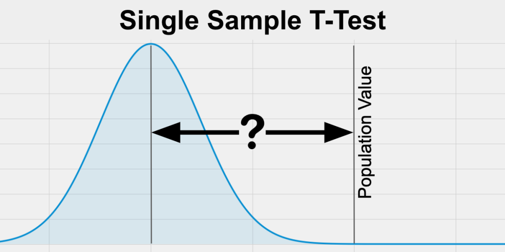
One Sample t-test: This test is used to determine whether the sample mean is significantly different from the hypothesized mean of the population.

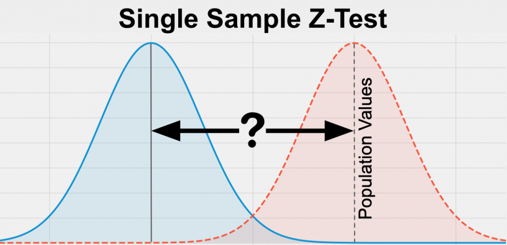
One Sample z-test: This test is used to determine whether the sample mean is significantly different from the hypothesized mean of the population when the population standard deviation is known.

Two Sample Hypothesis Tests

In a two-sample hypothesis test, a researcher collects data from two different populations and compares them to each other. The null hypothesis typically assumes that there is no significant difference between the two populations, and the researcher performs a statistical test to determine whether the observed difference is statistically significant. Some examples of two sample hypothesis tests are:

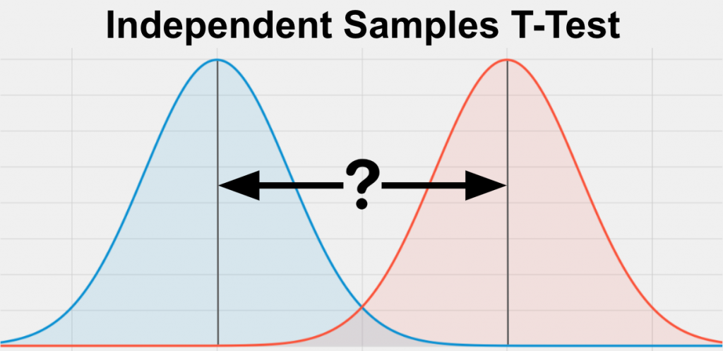
Independent Samples t-test: This test is used to compare the means of two independent samples to determine whether they are significantly different from each other.

Paired Samples t-test: This test is used to compare the means of two related samples, such as pre-test and post-test scores of the same group of subjects.

Figure: https://statstest.b-cdn.net/wp-content/uploads/2020/10/Paired-Samples-T-Test.jpg

In summary, one-sample hypothesis tests are used to test hypotheses about a single population, while two-sample hypothesis tests are used to compare two populations. The appropriate test to use depends on the nature of the data and the research question being investigated.

Steps of Hypothesis Testing

Hypothesis testing involves a series of steps that help researchers determine whether there is enough evidence to support or reject a hypothesis. These steps can be broadly classified into four categories:

Formulating the Hypothesis

The first step in hypothesis testing is to formulate the null hypothesis and alternative hypothesis. The null hypothesis usually assumes that there is no significant difference between two variables, while the alternative hypothesis suggests the presence of a relationship or difference. It is important to formulate clear and testable hypotheses before proceeding with data collection.

Collecting Data

The second step is to collect relevant data that can be used to test the hypotheses. The data collection process should be carefully designed to ensure that the sample is representative of the population of interest. The sample size should be large enough to produce statistically valid results.

Analyzing Data

The third step is to analyze the data using appropriate statistical tests. The choice of test depends on the nature of the data and the research question being investigated. The results of the statistical analysis will provide information on whether the null hypothesis can be rejected in favor of the alternative hypothesis.

Interpreting Results

The final step is to interpret the results of the statistical analysis. The researcher needs to determine whether the results are statistically significant and whether they support or reject the hypothesis. The researcher should also consider the limitations of the study and the potential implications of the results.

Common Errors in Hypothesis Testing

Hypothesis testing is a statistical method used to determine if there is enough evidence to support or reject a specific hypothesis about a population parameter based on a sample of data. The two types of errors that can occur in hypothesis testing are:

Type I error: This occurs when the researcher rejects the null hypothesis even though it is true. Type I error is also known as a false positive.

Type II error: This occurs when the researcher fails to reject the null hypothesis even though it is false. Type II error is also known as a false negative.

To minimize these errors, it is important to carefully design and conduct the study, choose appropriate statistical tests, and properly interpret the results. Researchers should also acknowledge the limitations of their study and consider the potential sources of error when drawing conclusions.

Null and Alternative Hypotheses

In hypothesis testing, there are two types of hypotheses: null hypothesis and alternative hypothesis.

The Null Hypothesis

The null hypothesis (H0) is a statement that assumes there is no significant difference or relationship between two variables. It is the default hypothesis that is assumed to be true until there is sufficient evidence to reject it. The null hypothesis is often written as a statement of equality, such as “the mean of Group A is equal to the mean of Group B.”

The Alternative Hypothesis

The alternative hypothesis (Ha) is a statement that suggests the presence of a significant difference or relationship between two variables. It is the hypothesis that the researcher is interested in testing. The alternative hypothesis is often written as a statement of inequality, such as “the mean of Group A is not equal to the mean of Group B.”

The null and alternative hypotheses are complementary and mutually exclusive. If the null hypothesis is rejected, the alternative hypothesis is accepted. If the null hypothesis cannot be rejected, the alternative hypothesis is not supported.

It is important to note that the null hypothesis is not necessarily true. It is simply a statement that assumes there is no significant difference or relationship between the variables being studied. The purpose of hypothesis testing is to determine whether there is sufficient evidence to reject the null hypothesis in favor of the alternative hypothesis.

Significance Level and P Value

In hypothesis testing, the significance level (alpha) is the probability of making a Type I error, which is rejecting the null hypothesis when it is actually true. The most commonly used significance level in scientific research is 0.05, meaning that there is a 5% chance of making a Type I error.

The p-value is a statistical measure that indicates the probability of obtaining the observed results or more extreme results if the null hypothesis is true. It is a measure of the strength of evidence against the null hypothesis. A small p-value (typically less than the chosen significance level of 0.05) suggests that there is strong evidence against the null hypothesis, while a large p-value suggests that there is not enough evidence to reject the null hypothesis.

If the p-value is less than the significance level (p < alpha), then the null hypothesis is rejected and the alternative hypothesis is accepted. This means that there is sufficient evidence to suggest that there is a significant difference or relationship between the variables being studied. On the other hand, if the p-value is greater than the significance level (p > alpha), then the null hypothesis is not rejected and the alternative hypothesis is not supported.

If you want an easy-to-understand summary of the significance level, you will find it in this article: An easy-to-understand summary of significance level .

It is important to note that statistical significance does not necessarily imply practical significance or importance. A small difference or relationship between variables may be statistically significant but may not be practically significant. Additionally, statistical significance depends on sample size and effect size, among other factors, and should be interpreted in the context of the study design and research question.

Power Analysis for Hypothesis Testing

Power analysis is a statistical method used in hypothesis testing to determine the sample size needed to detect a specific effect size with a certain level of confidence. The power of a statistical test is the probability of correctly rejecting the null hypothesis when it is false or the probability of avoiding a Type II error.

Power analysis is important because it helps researchers determine the appropriate sample size needed to achieve a desired level of power. A study with low power may fail to detect a true effect, leading to a Type II error, while a study with high power is more likely to detect a true effect, leading to more accurate and reliable results.

To conduct a power analysis, researchers need to specify the desired power level, significance level, effect size, and sample size. Effect size is a measure of the magnitude of the difference or relationship between variables being studied, and is typically estimated from previous research or pilot studies. The power analysis can then determine the necessary sample size needed to achieve the desired power level.

Power analysis can also be used retrospectively to determine the power of a completed study, based on the sample size, effect size, and significance level. This can help researchers evaluate the strength of their conclusions and determine whether additional research is needed.

Overall, power analysis is an important tool in hypothesis testing, as it helps researchers design studies that are adequately powered to detect true effects and avoid Type II errors

Bayesian Hypothesis Testing

Bayesian hypothesis testing is a statistical method that allows researchers to evaluate the evidence for and against competing hypotheses, based on the likelihood of the observed data under each hypothesis, as well as the prior probability of each hypothesis. Unlike classical hypothesis testing, which focuses on rejecting null hypotheses based on p-values, Bayesian hypothesis testing provides a more nuanced and informative approach to hypothesis testing, by allowing researchers to quantify the strength of evidence for and against each hypothesis.

In Bayesian hypothesis testing, researchers start with a prior probability distribution for each hypothesis, based on existing knowledge or beliefs. They then update the prior probability distribution based on the likelihood of the observed data under each hypothesis, using Bayes’ theorem. The resulting posterior probability distribution represents the probability of each hypothesis, given the observed data.

The strength of evidence for one hypothesis versus another can be quantified by calculating the Bayes factor, which is the ratio of the likelihood of the observed data under one hypothesis versus another, weighted by their prior probabilities. A Bayes factor greater than 1 indicates evidence in favor of one hypothesis, while a Bayes factor less than 1 indicates evidence in favor of the other hypothesis.

Bayesian hypothesis testing has several advantages over classical hypothesis testing. First, it allows researchers to update their prior beliefs based on observed data, which can lead to more accurate and reliable conclusions. Second, it provides a more informative measure of evidence than p-values, which only indicate whether the observed data is statistically significant at a predetermined level. Finally, it can accommodate complex models with multiple parameters and hypotheses, which may be difficult to analyze using classical methods.

Overall, Bayesian hypothesis testing is a powerful and flexible statistical method that can help researchers make more informed decisions and draw more accurate conclusions from their data.

Make scientifically accurate infographics in minutes

Mind the Graph platform is a powerful tool that helps scientists create scientifically accurate infographics in an easy way. With its intuitive interface, customizable templates, and extensive library of scientific illustrations and icons, Mind the Graph makes it easy for researchers to create professional-looking graphics that effectively communicate their findings to a broader audience.

Subscribe to our newsletter

Exclusive high quality content about effective visual communication in science.

Unlock Your Creativity

Create infographics, presentations and other scientifically-accurate designs without hassle — absolutely free for 7 days!

Content tags

• school Campus Bookshelves
• menu_book Bookshelves
• perm_media Learning Objects
• login Login
• how_to_reg Request Instructor Account
• hub Instructor Commons

Margin Size

• Download Page (PDF)
• Download Full Book (PDF)
• Periodic Table
• Physics Constants
• Scientific Calculator
• Reference & Cite
• Tools expand_more
• Readability

selected template will load here

This action is not available.

9: Hypothesis Testing

• Last updated
• Save as PDF
• Page ID 10210

• Kyle Siegrist
• University of Alabama in Huntsville via Random Services

\( \newcommand{\vecs}[1]{\overset { \scriptstyle \rightharpoonup} {\mathbf{#1}} } \)

\( \newcommand{\vecd}[1]{\overset{-\!-\!\rightharpoonup}{\vphantom{a}\smash {#1}}} \)

\( \newcommand{\id}{\mathrm{id}}\) \( \newcommand{\Span}{\mathrm{span}}\)

( \newcommand{\kernel}{\mathrm{null}\,}\) \( \newcommand{\range}{\mathrm{range}\,}\)

\( \newcommand{\RealPart}{\mathrm{Re}}\) \( \newcommand{\ImaginaryPart}{\mathrm{Im}}\)

\( \newcommand{\Argument}{\mathrm{Arg}}\) \( \newcommand{\norm}[1]{\| #1 \|}\)

\( \newcommand{\inner}[2]{\langle #1, #2 \rangle}\)

\( \newcommand{\Span}{\mathrm{span}}\)

\( \newcommand{\id}{\mathrm{id}}\)

\( \newcommand{\kernel}{\mathrm{null}\,}\)

\( \newcommand{\range}{\mathrm{range}\,}\)

\( \newcommand{\RealPart}{\mathrm{Re}}\)

\( \newcommand{\ImaginaryPart}{\mathrm{Im}}\)

\( \newcommand{\Argument}{\mathrm{Arg}}\)

\( \newcommand{\norm}[1]{\| #1 \|}\)

\( \newcommand{\Span}{\mathrm{span}}\) \( \newcommand{\AA}{\unicode[.8,0]{x212B}}\)

\( \newcommand{\vectorA}[1]{\vec{#1}}      % arrow\)

\( \newcommand{\vectorAt}[1]{\vec{\text{#1}}}      % arrow\)

\( \newcommand{\vectorB}[1]{\overset { \scriptstyle \rightharpoonup} {\mathbf{#1}} } \)

\( \newcommand{\vectorC}[1]{\textbf{#1}} \)

\( \newcommand{\vectorD}[1]{\overrightarrow{#1}} \)

\( \newcommand{\vectorDt}[1]{\overrightarrow{\text{#1}}} \)

\( \newcommand{\vectE}[1]{\overset{-\!-\!\rightharpoonup}{\vphantom{a}\smash{\mathbf {#1}}}} \)

Hypothesis testing refers to the process of choosing between competing hypotheses about a probability distribution, based on observed data from the distribution. It is a core topic in mathematical statistics, and indeed is a fundamental part of the language of statistics. In this chapter, we study the basics of hypothesis testing, and explore hypothesis tests in some of the most important parametric models: the normal model and the Bernoulli model.

• 9.1: Introduction to Hypothesis Testing In hypothesis testing, the goal is to see if there is sufficient statistical evidence to reject a presumed null hypothesis in favor of a conjectured alternative hypothesis.
• 9.2: Tests in the Normal Model
• 9.3: Tests in the Bernoulli Model
• 9.4: Tests in the Two-Sample Normal Model
• 9.5: Likelihood Ratio Tests
• 9.6: Chi-Square Tests

Help | Advanced Search

Physics > Data Analysis, Statistics and Probability

Title: statistical divergences in high-dimensional hypothesis testing and a modern technique for estimating them.

Abstract: Hypothesis testing in high dimensional data is a notoriously difficult problem without direct access to competing models' likelihood functions. This paper argues that statistical divergences can be used to quantify the difference between the population distributions of observed data and competing models, justifying their use as the basis of a hypothesis test. We go on to point out how modern techniques for functional optimization let us estimate many divergences, without the need for population likelihood functions, using samples from two distributions alone. We use a physics-based example to show how the proposed two-sample test can be implemented in practice, and discuss the necessary steps required to mature the ideas presented into an experimental framework.

Submission history

Access paper:.

• Other Formats

References & Citations

• INSPIRE HEP
• Google Scholar
• Semantic Scholar

BibTeX formatted citation

Bibliographic and Citation Tools

Code, data and media associated with this article, recommenders and search tools.

• Institution

arXivLabs: experimental projects with community collaborators

arXivLabs is a framework that allows collaborators to develop and share new arXiv features directly on our website.

Both individuals and organizations that work with arXivLabs have embraced and accepted our values of openness, community, excellence, and user data privacy. arXiv is committed to these values and only works with partners that adhere to them.

Have an idea for a project that will add value for arXiv's community? Learn more about arXivLabs .

• School Guide
• Mathematics
• Number System and Arithmetic
• Trigonometry
• Probability
• Mensuration
• Maths Formulas
• Class 8 Maths Notes
• Class 9 Maths Notes
• Class 10 Maths Notes
• Class 11 Maths Notes
• Class 12 Maths Notes
• Data Analysis with Python

Introduction to Data Analysis

• What is Data Analysis?
• Data Analytics and its type
• How to Install Numpy on Windows?
• How to Install Pandas in Python?
• How to Install Matplotlib on python?
• How to Install Python Tensorflow in Windows?

Data Analysis Libraries

• Pandas Tutorial
• NumPy Tutorial - Python Library
• Data Analysis with SciPy
• Introduction to TensorFlow

Data Visulization Libraries

• Matplotlib Tutorial
• Python Seaborn Tutorial
• Plotly tutorial
• Introduction to Bokeh in Python

Exploratory Data Analysis (EDA)

• Univariate, Bivariate and Multivariate data and its analysis
• Measures of Central Tendency in Statistics
• Measures of spread - Range, Variance, and Standard Deviation
• Interquartile Range and Quartile Deviation using NumPy and SciPy
• Anova Formula
• Skewness of Statistical Data
• How to Calculate Skewness and Kurtosis in Python?
• Difference Between Skewness and Kurtosis
• Histogram | Meaning, Example, Types and Steps to Draw
• Interpretations of Histogram
• Quantile Quantile plots
• What is Univariate, Bivariate & Multivariate Analysis in Data Visualisation?
• Using pandas crosstab to create a bar plot
• Exploring Correlation in Python
• Mathematics | Covariance and Correlation
• Factor Analysis | Data Analysis
• Data Mining - Cluster Analysis
• MANOVA Test in R Programming
• Python - Central Limit Theorem
• Probability Distribution Function
• Probability Density Estimation & Maximum Likelihood Estimation
• Exponential Distribution in R Programming - dexp(), pexp(), qexp(), and rexp() Functions
• Mathematics | Probability Distributions Set 4 (Binomial Distribution)
• Poisson Distribution - Definition, Formula, Table and Examples
• P-Value: Comprehensive Guide to Understand, Apply, and Interpret
• Z-Score in Statistics
• How to Calculate Point Estimates in R?
• Confidence Interval
• Chi-square test in Machine Learning

Understanding Hypothesis Testing

Data preprocessing.

• ML | Data Preprocessing in Python
• ML | Overview of Data Cleaning
• ML | Handling Missing Values
• Detect and Remove the Outliers using Python

Data Transformation

• Data Normalization Machine Learning
• Sampling distribution Using Python

Time Series Data Analysis

• Data Mining - Time-Series, Symbolic and Biological Sequences Data
• Basic DateTime Operations in Python
• Time Series Analysis & Visualization in Python
• How to deal with missing values in a Timeseries in Python?
• How to calculate MOVING AVERAGE in a Pandas DataFrame?
• What is a trend in time series?
• How to Perform an Augmented Dickey-Fuller Test in R
• AutoCorrelation

Case Studies and Projects

• Top 8 Free Dataset Sources to Use for Data Science Projects
• Step by Step Predictive Analysis - Machine Learning
• 6 Tips for Creating Effective Data Visualizations

Hypothesis testing involves formulating assumptions about population parameters based on sample statistics and rigorously evaluating these assumptions against empirical evidence. This article sheds light on the significance of hypothesis testing and the critical steps involved in the process.

What is Hypothesis Testing?

Hypothesis testing is a statistical method that is used to make a statistical decision using experimental data. Hypothesis testing is basically an assumption that we make about a population parameter. It evaluates two mutually exclusive statements about a population to determine which statement is best supported by the sample data. 

Example: You say an average height in the class is 30 or a boy is taller than a girl. All of these is an assumption that we are assuming, and we need some statistical way to prove these. We need some mathematical conclusion whatever we are assuming is true.

Defining Hypotheses

Key Terms of Hypothesis Testing

• P-value: The P value , or calculated probability, is the probability of finding the observed/extreme results when the null hypothesis(H0) of a study-given problem is true. If your P-value is less than the chosen significance level then you reject the null hypothesis i.e. accept that your sample claims to support the alternative hypothesis.
• Test Statistic: The test statistic is a numerical value calculated from sample data during a hypothesis test, used to determine whether to reject the null hypothesis. It is compared to a critical value or p-value to make decisions about the statistical significance of the observed results.
• Critical value : The critical value in statistics is a threshold or cutoff point used to determine whether to reject the null hypothesis in a hypothesis test.
• Degrees of freedom: Degrees of freedom are associated with the variability or freedom one has in estimating a parameter. The degrees of freedom are related to the sample size and determine the shape.

Why do we use Hypothesis Testing?

Hypothesis testing is an important procedure in statistics. Hypothesis testing evaluates two mutually exclusive population statements to determine which statement is most supported by sample data. When we say that the findings are statistically significant, thanks to hypothesis testing. 

One-Tailed and Two-Tailed Test

One tailed test focuses on one direction, either greater than or less than a specified value. We use a one-tailed test when there is a clear directional expectation based on prior knowledge or theory. The critical region is located on only one side of the distribution curve. If the sample falls into this critical region, the null hypothesis is rejected in favor of the alternative hypothesis.

One-Tailed Test

There are two types of one-tailed test:

Two-Tailed Test

A two-tailed test considers both directions, greater than and less than a specified value.We use a two-tailed test when there is no specific directional expectation, and want to detect any significant difference.

What are Type 1 and Type 2 errors in Hypothesis Testing?

In hypothesis testing, Type I and Type II errors are two possible errors that researchers can make when drawing conclusions about a population based on a sample of data. These errors are associated with the decisions made regarding the null hypothesis and the alternative hypothesis.

How does Hypothesis Testing work?

Step 1: define null and alternative hypothesis.

We first identify the problem about which we want to make an assumption keeping in mind that our assumption should be contradictory to one another, assuming Normally distributed data.

Step 2 – Choose significance level

Step 3 – Collect and Analyze data.

Gather relevant data through observation or experimentation. Analyze the data using appropriate statistical methods to obtain a test statistic.

Step 4-Calculate Test Statistic

The data for the tests are evaluated in this step we look for various scores based on the characteristics of data. The choice of the test statistic depends on the type of hypothesis test being conducted.

There are various hypothesis tests, each appropriate for various goal to calculate our test. This could be a Z-test , Chi-square , T-test , and so on.

• Z-test : If population means and standard deviations are known. Z-statistic is commonly used.
• t-test : If population standard deviations are unknown. and sample size is small than t-test statistic is more appropriate.
• Chi-square test : Chi-square test is used for categorical data or for testing independence in contingency tables
• F-test : F-test is often used in analysis of variance (ANOVA) to compare variances or test the equality of means across multiple groups.

We have a smaller dataset, So, T-test is more appropriate to test our hypothesis.

T-statistic is a measure of the difference between the means of two groups relative to the variability within each group. It is calculated as the difference between the sample means divided by the standard error of the difference. It is also known as the t-value or t-score.

Step 5 – Comparing Test Statistic:

In this stage, we decide where we should accept the null hypothesis or reject the null hypothesis. There are two ways to decide where we should accept or reject the null hypothesis.

Method A: Using Crtical values

Comparing the test statistic and tabulated critical value we have,

• If Test Statistic>Critical Value: Reject the null hypothesis.
• If Test Statistic≤Critical Value: Fail to reject the null hypothesis.

Note: Critical values are predetermined threshold values that are used to make a decision in hypothesis testing. To determine critical values for hypothesis testing, we typically refer to a statistical distribution table , such as the normal distribution or t-distribution tables based on.

Method B: Using P-values

We can also come to an conclusion using the p-value,

Note : The p-value is the probability of obtaining a test statistic as extreme as, or more extreme than, the one observed in the sample, assuming the null hypothesis is true. To determine p-value for hypothesis testing, we typically refer to a statistical distribution table , such as the normal distribution or t-distribution tables based on.

Step 7- Interpret the Results

At last, we can conclude our experiment using method A or B.

Calculating test statistic

To validate our hypothesis about a population parameter we use statistical functions . We use the z-score, p-value, and level of significance(alpha) to make evidence for our hypothesis for normally distributed data .

1. Z-statistics:

When population means and standard deviations are known.

• μ represents the population mean, 
• σ is the standard deviation
• and n is the size of the sample.

2. T-Statistics

T test is used when n<30,

t-statistic calculation is given by:

• t = t-score,
• x̄ = sample mean
• μ = population mean,
• s = standard deviation of the sample,
• n = sample size

3. Chi-Square Test

Chi-Square Test for Independence categorical Data (Non-normally distributed) using:

• i,j are the rows and columns index respectively.

Real life Hypothesis Testing example

Let’s examine hypothesis testing using two real life situations,

Case A: D oes a New Drug Affect Blood Pressure?

Imagine a pharmaceutical company has developed a new drug that they believe can effectively lower blood pressure in patients with hypertension. Before bringing the drug to market, they need to conduct a study to assess its impact on blood pressure.

• Before Treatment: 120, 122, 118, 130, 125, 128, 115, 121, 123, 119
• After Treatment: 115, 120, 112, 128, 122, 125, 110, 117, 119, 114

Step 1 : Define the Hypothesis

• Null Hypothesis : (H 0 )The new drug has no effect on blood pressure.
• Alternate Hypothesis : (H 1 )The new drug has an effect on blood pressure.

Step 2: Define the Significance level

Let’s consider the Significance level at 0.05, indicating rejection of the null hypothesis.

If the evidence suggests less than a 5% chance of observing the results due to random variation.

Step 3 : Compute the test statistic

Using paired T-test analyze the data to obtain a test statistic and a p-value.

The test statistic (e.g., T-statistic) is calculated based on the differences between blood pressure measurements before and after treatment.

t = m/(s/√n)

• m  = mean of the difference i.e X after, X before
• s  = standard deviation of the difference (d) i.e d i ​= X after, i ​− X before,
• n  = sample size,

then, m= -3.9, s= 1.8 and n= 10

we, calculate the , T-statistic = -9 based on the formula for paired t test

Step 4: Find the p-value

The calculated t-statistic is -9 and degrees of freedom df = 9, you can find the p-value using statistical software or a t-distribution table.

thus, p-value = 8.538051223166285e-06

Step 5: Result

• If the p-value is less than or equal to 0.05, the researchers reject the null hypothesis.
• If the p-value is greater than 0.05, they fail to reject the null hypothesis.

Conclusion: Since the p-value (8.538051223166285e-06) is less than the significance level (0.05), the researchers reject the null hypothesis. There is statistically significant evidence that the average blood pressure before and after treatment with the new drug is different.

Python Implementation of Hypothesis Testing

Let’s create hypothesis testing with python, where we are testing whether a new drug affects blood pressure. For this example, we will use a paired T-test. We’ll use the scipy.stats library for the T-test.

Scipy is a mathematical library in Python that is mostly used for mathematical equations and computations.

We will implement our first real life problem via python,

In the above example, given the T-statistic of approximately -9 and an extremely small p-value, the results indicate a strong case to reject the null hypothesis at a significance level of 0.05. 

• The results suggest that the new drug, treatment, or intervention has a significant effect on lowering blood pressure.
• The negative T-statistic indicates that the mean blood pressure after treatment is significantly lower than the assumed population mean before treatment.

Case B : Cholesterol level in a population

Data: A sample of 25 individuals is taken, and their cholesterol levels are measured.

Cholesterol Levels (mg/dL): 205, 198, 210, 190, 215, 205, 200, 192, 198, 205, 198, 202, 208, 200, 205, 198, 205, 210, 192, 205, 198, 205, 210, 192, 205.

Populations Mean = 200

Population Standard Deviation (σ): 5 mg/dL(given for this problem)

Step 1: Define the Hypothesis

• Null Hypothesis (H 0 ): The average cholesterol level in a population is 200 mg/dL.
• Alternate Hypothesis (H 1 ): The average cholesterol level in a population is different from 200 mg/dL.

As the direction of deviation is not given , we assume a two-tailed test, and based on a normal distribution table, the critical values for a significance level of 0.05 (two-tailed) can be calculated through the z-table and are approximately -1.96 and 1.96.

Step 4: Result

Since the absolute value of the test statistic (2.04) is greater than the critical value (1.96), we reject the null hypothesis. And conclude that, there is statistically significant evidence that the average cholesterol level in the population is different from 200 mg/dL

Limitations of Hypothesis Testing

• Although a useful technique, hypothesis testing does not offer a comprehensive grasp of the topic being studied. Without fully reflecting the intricacy or whole context of the phenomena, it concentrates on certain hypotheses and statistical significance.
• The accuracy of hypothesis testing results is contingent on the quality of available data and the appropriateness of statistical methods used. Inaccurate data or poorly formulated hypotheses can lead to incorrect conclusions.
• Relying solely on hypothesis testing may cause analysts to overlook significant patterns or relationships in the data that are not captured by the specific hypotheses being tested. This limitation underscores the importance of complimenting hypothesis testing with other analytical approaches.

Hypothesis testing stands as a cornerstone in statistical analysis, enabling data scientists to navigate uncertainties and draw credible inferences from sample data. By systematically defining null and alternative hypotheses, choosing significance levels, and leveraging statistical tests, researchers can assess the validity of their assumptions. The article also elucidates the critical distinction between Type I and Type II errors, providing a comprehensive understanding of the nuanced decision-making process inherent in hypothesis testing. The real-life example of testing a new drug’s effect on blood pressure using a paired T-test showcases the practical application of these principles, underscoring the importance of statistical rigor in data-driven decision-making.

Frequently Asked Questions (FAQs)

1. what are the 3 types of hypothesis test.

There are three types of hypothesis tests: right-tailed, left-tailed, and two-tailed. Right-tailed tests assess if a parameter is greater, left-tailed if lesser. Two-tailed tests check for non-directional differences, greater or lesser.

2.What are the 4 components of hypothesis testing?

Null Hypothesis ( ): No effect or difference exists. Alternative Hypothesis ( ): An effect or difference exists. Significance Level ( ): Risk of rejecting null hypothesis when it’s true (Type I error). Test Statistic: Numerical value representing observed evidence against null hypothesis.

3.What is hypothesis testing in ML?

Statistical method to evaluate the performance and validity of machine learning models. Tests specific hypotheses about model behavior, like whether features influence predictions or if a model generalizes well to unseen data.

4.What is the difference between Pytest and hypothesis in Python?

Pytest purposes general testing framework for Python code while Hypothesis is a Property-based testing framework for Python, focusing on generating test cases based on specified properties of the code.

Please Login to comment...

Similar reads.

• data-science
• Data Science
• Machine Learning

Improve your Coding Skills with Practice

What kind of Experience do you want to share?

The role of environmental tax on the environmental quality in EU counties: evidence from panel vector autoregression approach

• Research Article
• Open access
• Published: 14 May 2024

Cite this article

You have full access to this open access article

• Buket Savranlar 1 ,
• Seyyid Ali Ertas 2 &
• Alper Aslan   ORCID: orcid.org/0000-0003-1408-0921 3  

This study intends to analyze the influence of environmental taxes on pollution in EU-27 nations. Furthermore, energy from renewable sources consumption and urbanization are employed to clarify CO 2 emissions in this study that tests the EKC hypothesis. According to the findings, an increase in environmental taxes reduces CO 2 emissions by 0.14%. Also, the data supported the validity of the EKC concept. The findings of the causality test demonstrated that there is a bidirectional causal link between CO 2 emissions and environmental taxes. These results reflect that environmental tax revenues contribute to sustainability as an effective policy tool in EU countries. Policies regarding environmental tax enforcement come to the fore in terms of both keeping the balance in economic activities and serving sustainability.

Avoid common mistakes on your manuscript.

Introduction

Environmental issues such as global warming with air pollution, global climate change, and biodiversity reduction are within the main scope and impact of the economy. The quality of the air and the protection of the environment, which are environmental elements, are an important public commodity (Theeuwes 1991 :67–68; He et al. 2018 :7456). Reducing air pollution and therefore improving the quality of air can be treated as a national public commodity with no competition in its consumption and inability to exclude it. Because of this dimension of publicity, countries have various responsibilities in solving environmental problems and improving environmental quality. Accordingly, countries develop policies to ensure and sustain the environment, while also having a regulatory function through regulations, especially in the elimination of environmental negative externalities. All around the world, air pollution has been linked to health issues for people (Lelieveld et al. 2015 ; Cohen et al. 2017 ; Heft-Neal et al. 2018 ). PM 2:5 , which might permeate profoundly entering the bloodstream and respiratory system, leading to illnesses (Lelieveld c., 2015 ; Li et al. 2019 ), is the principal source of air pollution. Climate change is the most serious environmental issue that humanity has ever faced Change I P O C ( 2001 ). The earth’s surface temperature has been rising over the past 30 years. The dangers of major detrimental consequences on human life, property, the economy, and the environment have considerably grown as global warming rates and amplitudes continue to rise.

The major component of greenhouse gas emissions is CO2. CO2 emissions from economic activities, particularly conventional patterns of energy use based mostly on non-renewable, have become the principal human driver driving global warming from a global viewpoint (Meinshausen et al. 2009 ; Sari and Soytas 2009 ). When compared to 2005, worldwide CO2 emissions increased by around 5 109 tons in 2015. CO2 emissions in wealthy nations decreased by 1:1 109 tons, whereas those in developing nations climbed by 6:1 109 tons, essentially canceling out the developed countries’ emission reduction efforts (BP 2016 ). Developing nations emit enormous amounts of CO2 because of their aggressive promotion of industrialization and urbanization. Developing countries would endure more severe environmental damage and climate change repercussions than developed countries. More than 170 nations agreed to the Paris Agreement in 2016, pledging to work toward a long-term objective of keeping global warming to 2 degrees Celsius or less. It is critical to examine variations in global Carbon emissions to achieve this aim. Environmental Two factors determine the quality of the air: first, the direct output of human production activities, which are the primary causes of pollution and include economic expansion (Li et al. 2019 ), industrialization development (Gan et al. 2018 ), and energy use (Khan et al. 2019 ). In addition to this, excessive emissions and inadequate environmental spending will result in a decline in air quality.

At this point, the effects of regulating environmental stewardship are investigated using a variety of methodologies (Laplante and Ristone 1996 ) emphasizing three distinct perspectives: (1) Blackman and Kildegaard ( 2010 ) investigate environmental agency safety checks in Mexico and obtain that regulatory stress is unrelated to reducing pollution; According to (2) Lanoie et al. ( 2011 ), regulations will make it more expensive for companies to minimize pollution and release, drive away valuable resources, and lower efficiency and market competitiveness, making environmental issues unmanageable. By global cooperation, agreements for the solution of environmental problems have been raised, the negative effects and negative effects of environmental pollution have become a concern in the social sphere, the causes and consequences of pollution have been the focus of research in academic circles, and ways to improve the quality of the air have been discussed in the prevention and reduction of pollution.

Only a few academics have highlighted concerns regarding environmental taxes. Using the variance (DID) approach, Lin and Li ( 2011 ) studied the effects of carbon pricing on governance systems in five Northern countries. Many studies investigated the various aspects of a carbon tax. Lin and Li ( 2011 ) discovered that while the carbon price lowered CO 2 emissions substantially in Finland, the effects were significantly negative in Denmark and Sweden. The majority of academics still think that environmental levies improve environmental governance. González and Hosoda ( 2016 ) used a Bayesian structure time series model to assess the impact of an aviation oil fuel tax on national transportation consumption growth in Japan, and they discovered that the tax decreased Emissions of CO 2 by planes. In this context, agreements for solving environmental problems have been raised by global cooperation, the negative effects and negatives created by environmental pollution in the social sphere have become a concern, and in academic circles, the causes and consequences of pollution have been the subject of research and ways to prevent and reduce pollution have been discussed.

In keeping with the emissions and sustainable development targets, there has been a discernible growth in environmental pollution taxes inside the European Union (EU). The goal of taxation is to reduce carbon emissions to a manageable 5%. Energy, environment, and transportation taxes are among the taxes imposed for this purpose, particularly in Slovenia, Poland, France, Portugal, Finland, Latvia, Ireland, and Denmark. The EU is taking what are arguably the most obvious actions in the world in this regard. To lessen the detrimental externalities that third parties produce in production and consumption, the EU has imposed emission and environmental fees. Pollution, land degradation, and the greenhouse effect which raises living standards, lowers product quality, lowers income, and consumes more energy are examples of negative externalities.

More work is needed to regulate the release of toxic compounds into the atmosphere to safeguard the sustainability of ecosystem services, and the well-being of European populations, and prevent hazardous disruption of the global climate system. Numerous strategies are theoretically possible to further lower pollution in the future. For instance, one of its main objectives might be to lower environmental pollution and raise air quality through the usage of environmental levies.

Ecological taxation aims to transfer the tax burden from economically desirable social goods, such as jobs, income, and investments, to economically undesirable social goods, such as waste and environmental damage (Bosquet 2000 ). In addition, environmental taxes have nearly also been set at a lower level than what is warranted by environmental damages in Europe and have instead been utilized to raise income. Is it reasonable to assess the environmental impact and economic efficiency of a tool whose primary objective is to generate revenue? Secondly, environmental taxes are not self-contained. In Europe, they are frequently used to supplement existing rules with standards and guidelines, and they are frequently utilized to accelerate the adoption of new technology. A fundamental challenge is separating the effects of environmental taxes from other forms of regulation that are in force at the same time.

Unlike previous research, this study has looked at how environmental taxes affect EU carbon emissions. The impact of urbanization and the use of renewable energy on emissions of carbon are investigated for this reason. To the best of our knowledge, this study used the panel VAR technique to investigate, for the first time, the impact of energy use, urbanization, and environmental levies on the quality of the environment for EU nations. Our analysis also contributes to the econometric structure. We must enforce the requirement that the fundamental framework be the same for every cross-section unit when using the VAR process on panel data. One method to get around the parameter limitation is to introduce the fixed effects that are depicted in the model to make room for “individual variability” in the variable values, as this restriction is likely to be broken in practice. The delays of the variables that are dependent link fixed effects to regressors; therefore, biased coefficients will result from the standard averaging approach used to remove fixed effects. We employ a forward mean difference, also known as the “Helmert procedure,” to get around this issue. Only the forward average—that is, the average of all future data that are accessible for each nation year—is eliminated by this process. We may employ lagged regression coefficients as tools and estimate the coefficients using the system GMM since this transformation maintains the orthogonality between the modified variables and the regressors (Love and Zicchino 2006 ).

The remaining research is organized as follows: The relevant empirical literature is presented in the “ Literature review ” section. The “Model specification, data and methodology” section explains the technique, model, and data. Empirical results are included in the “ Empirical findings ” section. Concluding thoughts and policy implications are presented in the “ Conclusion ” section.

Literature review

Scholars, policymakers, and economists have been debating the connections between energy usage, environmental quality, and taxes connected to the environment for the past thirty years. The single-country and multi-country data analysis situations covered in this literature review have received the majority of attention in the research that is currently accessible. After reviewing the literature, we can organize it into three broad categories since research has been done on topics like environmental taxes, consumption of energy and the economy, and the relationship between energy use and the environment.

Very recently, Bekun ( 2024 ) has examined the relationship between conventional energy use, agricultural practices, economic growth, and environmental sustainability in South Africa by using Pesaran’s Autoregressive distributed lag (ARDL) method, as well as the dynamic ARDL simulations method. To meet the study’s objectives, a carbon income function is fitted to annual frequency data from 1975 to 2020. Bekun observed that economic expansion, fossil fuel energy use, and agricultural activities all have a negative impact on environmental sustainability in South Africa, implying a trade-off between economic growth and environmental quality. Bekun ( 2022 ) studied how renewable and non-renewable energy, economic growth, and energy sector investment affect CO2 emissions in India. The long-run elasticity of the variables was determined using canonical cointegration regression (CCR), completely modified least squares (FMOLS), and dynamic least squares (DOLS). Granger causality analysis was employed to determine the direction of the causal relationship between the variables that were highlighted. The results of empirical regression indicate a negative correlation between renewable energy and CO 2 emissions. The long-run elasticity of the variables was determined using canonical cointegration regression (CCR), completely modified least squares (FMOLS), and dynamic least squares (DOLS), and the direction of the causal relationship between the highlighted variables was determined using Granger causality analysis. The results of empirical regression indicate a negative correlation between renewable energy and CO 2 emissions. Nadiri et al. ( 2024 ) identified carbon dioxide (CO2) emissions as the main cause of the urgent problem of environmental deterioration, endangering the sustainability of the environment worldwide, particularly the member states of the European Union (EU). The findings demonstrate that while globalization, eco-innovation, carbon taxes, and renewable energy all help to slow down environmental degradation, economic development also helps to lessen the problems associated with environmental sustainability in EU member states. Xu et al. ( 2023 ) gathered information from 287 cities between 2010 and 2019 to examine the mechanism behind the fee and determine its effect on lowering pollution. The findings indicate that the environmental tax had a major knock-on effect on sewage, waste gas, and solid waste emissions. This suggests that intergovernmental cooperation and regional collaboration can improve the implementation of environmental tax policies and their emission reduction effects. Dmytrenko et al. ( 2024 ) investigated the effects of environmental levies and stricter environmental regulations on greenhouse gas emissions in a sample of eight European nations from Central and Western Europe. Our findings indicate that only in Western Europe does the strictness of environmental regulations have a major impact. It is interesting to note that R&D spending ended up having the biggest impact on both groups. Guo and Wang ( 2018 ) used annual time series data from 1985 to 2014 to investigate the connection between Beijing, China’s carbon emissions and environmental regulations. The authors experimentally investigated the consequences of environmental legislation in Beijing using the Johansen Cointegration, VAR model, and impulsive reaction function methodologies. Environmental restrictions, according to the research, could help to foster technical development while also reducing the effects of carbon emissions. with relation to energy, the environment, the economy, and economic competitiveness. In a similar vein, Wolde-Rufael and Mulat-Weldemeskel ( 2022 ) discovered that environmental taxes and CO2 emissions in Latin American and Caribbean nations were negatively correlated. A similar conclusion was obtained about environmental taxes by Safi et al. ( 2021 ) after analyzing the impact of R&D and environmental taxes on carbon emissions in G7 nations. The impact of environmental tax measures on developing, developed, and growing nations was studied by Cottrell et al. ( 2015 ). Environmental fiscal policies that stray from the ideal tax design, according to the research, help to avert negative implications for international competition. The research argues that environment tax reform is a viable and affordable policy instrument for both long-term environmental conservation and economic prosperity. Morley ( 2012 ) examined the long-term impact of ecological tariffs on energy usage and pollutant emissions using data from 25 European nations between 1995 and 2005. The two-step GMM technique was used in this study to account for variability and unobserved heterogeneity difficulties in econometric assumptions. Environmental levies do not have a major impact on energy usage in the nations analyzed, according to the findings of the empirical research. Wang et al. ( 2015 ) used data from 36 Chinese industries to investigate the effects of carbon prices on industrial competitiveness. The authors conducted a thorough examination of the impact of carbon-related levies on various economic sectors. Fremstad and Paul ( 2019 ) looked at how carbon prices affect income disparity and general economic development in the United States. The authors came to the conclusion that the labor tax cuts associated with the carbon tax are being reduced, which is not enough to preserve Americans’ purchasing power. Peng et al. ( 2019 ) looked at how energy taxes might affect Jiangsu’s potential for prosperity and economy. Empirical research indicates that while energy taxes are advantageous for conserving resources and lowering energy usage, they also compromise economic and welfare goals. Rogan et al. ( 2011 ) investigated the impact of targeted policies on vehicle purchasing trends in the direction of lowering carbon-emitting automobiles. Drawing on statistics from Ireland, the authors concluded that at the start of a new taxing scheme, new-vehicle carbon emissions might be decreased by up to 13%. Ciaschini et al. ( 2012 ) assessed the relationship between taxes on the environment and carbon emissions from Italy using yearly time series data spanning from 2004 to 2007. The authors used an empirical general equilibrium technique (CGE) to hypothesize that tax policies might have an impact on regional prices, employment rates, economic growth, and carbon dioxide emissions. Miller and Vela ( 2013 ) investigated how environmental levies affected the reduction of pollutant emissions in fifty distinct nations. To test the key hypothesis, the researchers gathered annual data from 1995 to 2010 and used pass dynamics regression analysis. Stern et al. ( 1993 ) established a popular theoretical framework to explain pro-environmental behavior. They propose a social–psychology paradigm in which egoistic, social–altruistic, and biocentric value perspectives can all motivate impact on the environment. They next put the model to the test utilizing survey results. While they find widespread agreement for their approach, they also discover that only self-interested reasons are a true indicator of willingness to pay through taxes. The implicit pollution tax in the US quadrupled between 1990 and 2008, resulting in a 60% decrease in air pollutants from manufacturing industries despite a notable increase in industrial production (Shapiro and Walker 2018 ). However, other research has demonstrated that a carbon price has little effect on lowering carbon emissions (Klenert and Mattauch 2016 ; King et al. 2019 ).

Model specification, data, and methodology

This paper aims to analyze the effect of environmental taxation, economic growth, renewable energy, and urbanization on CO 2 emissions. The functional representation of this relationship is as follows:

This nexus is expressed as a panel data model as follows:

where i implies each unit of the panel (EU-27 countries Footnote 1 ), t denotes the data period (1995–2018). CO 2 is the dependent variable and implies CO 2 emissions in metric tons per capita. Independent variables are GDP per capita (constant 2015 US$), squared of GDP, environmental tax revenues (million dollars), the percentage of urban to total population, and the fraction of energy from renewable sources utilized for total final consumption of energy, respectively. The World Bank’s World Development Indicators provides other statistics, while the Eurostat database is the source of data for the environmental tax indicator. For every variable, the logarithmic transformation is utilized. Table 1 displays descriptive data for the series.

In this study, the panel vector autoregression (PVAR) method is adopted to estimate Eq. ( 2 ). Before estimating the equation, whether the variables contain a unit root is checked by both IPS test developed by Im et al. ( 2003 ) and CIPS panel unit root test developed by Pesaran ( 2007 ). The reason why these tests are preferred is that the IPS considers the heterogeneity of the panel and the CIPS test handled also the cross-section dependence. After the unit root testing, the procedure for the PVAR approach is followed.

The PVAR approach is developed by Abrigo and Love ( 2016 ). The estimation procedure of this method is based on the Generalized Method of Moments (GMM) approach. This method provides a detailed empirical evidence framework by enabling long-run coefficient estimation, causality analysis, variance decomposition analysis, and obtaining impulse-response graphs for the relationship under consideration. The main PVAR model is constructed as follows:

where \({X}_{pt}=\left[{CO2}_{pt},{GDP}_{pt}{,GDP2}_{pt},{TAX}_{pt},{REN}_{pt},{URB}_{pt}\right]\) implies a vector of the exogenous variables. \({Y}_{pt}\) is \(\left(kxk\right)\) vector of independent variables. \({\cup }_{c}\) is a vector of country-fixed effects and \({\mu }_{ct}\) is idiosyncratic error.

The PVAR approach considers unobserved heterogeneity and eliminates estimation errors caused by cross-sectional dependence panel VAR models add the cross-section to regular VAR models, but they are otherwise identical to standard VAR models in that each of the variables is endogenous and interdependent. The panel VAR method, however, has a few unique characteristics.

Due to the consideration of all endogenous variable delays, there is a dynamic interdependency between the variables. Additionally, error terms are typically associated across units; this characteristic is known as static interdependency.

Lastly, the shocks’ intercept, slope, and variance could vary depending on the unit. According to Canova and Ciccarelli ( 2013 ), this suggests that cross-sectional heterogeneity is available.

Empirical findings

In the first stage of the analysis, it is tested whether the series are stationary or not. Regarding this, both IPS and CIPS test results are presented in Table  2 . According to the IPS test results, it is understood that all variables are stationary at the first difference. When the results of the CIPS unit root test, which is another unit root testing approach adopted in this study, are examined, it is seen that the GDP , GDP 2 , and TAX variables are stationary at level, but others are stationary at first difference.

After the unit root tests, the panel VAR procedure is followed. First, the optimal lag length is determined, and the results are presented in Table  3 . According to Table  3 , it is concluded that the optimal lag length is 1 since the MBIC, MAIC, and MQIC have the lowest values at the lag(1).

The long-run coefficient estimates determined using lag(1) are shown in Table  4 . Because GDP has a positive influence on CO2 and GDP 2 has a negative impact on it, initial data show the presence of an inverted U-shaped link between economic growth and air pollution, supporting the validity of the EKC hypothesis in these nations. Another finding indicates that environmental fees improve the quality of the air in these nations. An increase in environmental taxes reduces CO 2 emissions by 0.14% in the European Union. This result is in line with Miller and Vela ( 2013 ), Guo and Wang ( 2018 ), Wolde-Rufael and Mulat-Weldemeskel ( 2022 ), Safi et al. ( 2021 ), Xu et al. ( 2023 ), and Nadiri et al. ( 2024 ). The findings regarding the relationship between environmental taxes and emissions may be evaluated in line with the widespread literature. This result confirms that the positive effects of environmental practices supported by strict policies are inevitable in the long run. On the other hand, the findings of Dmytrenko et al. ( 2024 ). Their results are important because they involve the comparison of two samples, central and western Europe. Since this study covers mostly Western European countries, it is compatible with their results for Western Europe. In fact, when the relevant literature and the results of this study are evaluated together, the success in the implementation of environmental taxes may be evaluated in connection with the institutional structure of the county or region and its success in public policies. Also, renewable energy consumption and urbanization have a negative impact on emissions, but this effect of renewable energy is statistically insignificant.

Empirical results show that environmental taxes are an effective policy tool in tackling the problem of negative environmental externalities in European countries. The main purpose of environmental taxes is to reduce pollution by preventing activities that are harmful to the environment. Therefore, the results reflect a taxation system that serves this purpose. Beyond this direct effect, another measure of the effectiveness of environmental taxes is that these taxes encourage companies to develop environmentally friendly technologies and consume renewable energy. In these countries, the positive effect of environmental tax on renewable energy consumption is another important finding, and the effectiveness of environmental tax becomes clearer at this point. Accordingly, an increase in environmental tax revenues increases renewable energy consumption by about 0.09% in the long run. Therefore, this result means that tax revenues are used for sustainable purposes. Unlike the positive contribution of environmental tax to air quality and renewable energy consumption, it is observed that it reduces economic growth, albeit slightly. Its negative effect on economic growth is that taxes are an element that increases the cost of companies and therefore reduces international competition.

According to other empirical findings, both renewable energy consumption and urbanization cause an increase in environmental tax revenues. An increase in renewable energy consumption increases environmental tax revenues by about 0.6%, while an increase in urbanization increases it by about 8%. It is an expected conclusion that environmental tax revenues increase with urbanization. It can be said that urbanization accelerates industrialization and accordingly production and consumption process and causes environmental sanctions such as taxes to become widespread in case they pose a threat to environmental quality. At this point, it is possible to explain the reducing effect of urbanization on emissions. Therefore, environmental tax practices caused by urbanization mean that tax revenues increase and these revenues are qualified as a source for environmentally friendly incentive practices. The fact that renewable energy consumption causes an increase in environmental tax revenues reflects the deviations from the environmentally friendly approach to renewable energy consumption.

Investigating the stability of the model discussed in the study is another stage of panel VAR analysis. The results of the stability test are presented both in Table  5 and graphically in Fig.  1 . The fact that all the results in Table  5 are less than 1 and therefore all the points in Fig.  1 are within the unit circle indicates that the model is stable. This result allows the analysis to be considered in more detail and the causality test to be performed in the next step. Causality test results are reported in Table  6 .

Stability of the PVAR model

The results of the causality test performed after the coefficient estimation point to some important findings. Accordingly, GDP and energy from renewable sources use have a one-way causal connection, as do emissions of carbon dioxide and renewable consumption of energy. Furthermore, bidirectional causation is shown between environmental tax and renewable energy use and urbanization, GDP and environmental tax and CO2 emissions, and so on. The causality test results support the interrelationships in the long-run coefficient estimation findings. Therefore, the strong links between emissions, environmental taxes, growth, clean energy consumption, and urbanization are emphasized once again. With this determination, in the next step, the variance decomposition between emissions and environmental tax is examined in the context of the main focus of the subject. The results obtained provide a significant inference.

Findings related to variance decomposition analysis are reported in Table  7 within the scope of emissions and environmental tax nexus. The first part of the table describes the change in emissions over 10 periods ahead through shocks in emissions and environmental tax. Accordingly, about 87% of changes in emissions are due to shocks in itself, while about 10% is caused by shocks in environmental taxes. In the second part of the table, changes in environmental taxes are explained by shocks in emissions and environmental tax. This part differs from the result in the first part of the table. Accordingly, the changes in environmental taxes over 10 periods ahead are explained by shocks in emissions of about 38%, while about 34% are explained by shocks in itself. Therefore, emissions have a critical role in the future of EU member countries as an important component that brings up the regulations regarding environmental tax.

The shocks and their effects in the variance decomposition analysis can be represented more comprehensively and clearly in the impulse-response functions. These functions with 95% confidence intervals are presented graphically in Fig.  2 . According to these results, the response of CO 2 emissions to a standard deviation shock in GDP is firstly positive and then negative. However, the response of emissions to a standard deviation shock in urbanization, renewable energy consumption, and environmental tax is firstly negative, and then positive.

Impulse-response graphs

This study examined the impact of economic development, urbanization, renewable energy usage, and environmental taxes on CO2 emissions in the EU-27. The PVAR technique was applied for this purpose between 1995 and 2018. The primary findings showed that urbanization, renewable energy use, and environmental taxes all had long-term detrimental effects on emissions. Additionally, the findings supported the EKC hypothesis’s validity in these nations.

In the light of the main findings, it is possible to make some policy implications for these countries. The results revealed that environmental taxes have a positive contribution to air quality more than renewable energy in these countries. However, considering that the growth-reducing effect of environmental taxes is greater than that of renewable energy consumption, the possible costs of environmental taxes should be reconsidered. At this point, it is necessary to complete the taxes applied for polluting sectors with a system that encourages the use of environmentally friendly technology to balance the costs. This means the development of a new reward-punishment approach in environmental regulations. One of the most critical points about taxes is the determination of tax rates. Accordingly, another important criterion is to determine the rates in polluting sectors by considering the sector-specific cost structures. With such an approach, a tax burden will be created that allows companies operating in related sectors to invest in environmentally friendly technologies. In these economies that are on the edge of economic, social, and democratic development, there is a suitable basis for more effective implementation of environmental taxes. Unless inactive choices (such as poverty) are made in the use of resources, developments such as environmental regulations in these countries produce positive results in favor of improving air quality.

In the following studies, factors such as economic growth, foreign trade, investment, poverty, democracy, corruption, and population can be considered the impact of environmental taxes on the effectiveness of environmental taxes, and the indirect effects of related factors on air quality, and how environmental taxes form the basis for the effectiveness of environmental taxes in developed and developing economies.

Data availability

The data used to support the findings of this study are included within the article.

Austria, Belgium, Bulgaria, Croatia, Cyprus, Czech Republic, Denmark, Estonia, Finland, France, Germany, Greece, Hungary, Ireland, Italy, Latvia, Lithuania, Luxembourg, Malta, Netherlands, Poland, Portugal, Romania, Slovak Republic, Slovenia, Spain, Sweden.

Abrigo MR, Love I (2016) Estimation of panel vector autoregression in Stata. Stata J 16(3):778–804

Azam M, Khan AQ (2016) Urbanization and environmental degradation: evidence from four SAARC countries Bangladesh, India, Pakistan, and Sri Lanka. Environ Prog Sustain Energy 35(3):823–832

Article   CAS   Google Scholar  

Bekun FV (2022) Mitigating emissions in India: accounting for the role of real income, renewable energy consumption and investment in energy. Int J Energy Econ Policy 12(1):188–192

Article   Google Scholar  

Bekun FV (2024) Race to carbon neutrality in South Africa: what role does environmental technological innovation play? Appl Energy 354:122212

Blackman A, Kildegaard A (2010) Clean technological change in developing country industrial clusters: Mexican leather tanning. Environ Econ Policy Stud 12:115–132

Bosquet B (2000) Environmental tax reform: does it work? A survey of the empirical evidence. Ecol Econ 34(1):19–32

British Petroleum Company (2016) BP statistical review of world energy. https://www.bp.com/content/dam/bp/pdf/energy-economics/statistical-review-2016/bp-statistical-review-of-world-energy-2016-full . Accessed 31 Mar 2024

Canova F, Ciccarelli M (2013) Panel vector autoregressive models: a survey. ECB Working Paper, No. 1507, European Central Bank (ECB), Frankfurt a. Available at SSRN: https://www.ssrn.com/abstract=2201610

Change I P O C (2001) Climate change 2007: impacts, adaptation and vulnerability. IPCC Sixth Assessment Report, Genebra, Suíça

Ciaschini M, Pretaroli R, Severini F, Socci C (2012) Regional double dividend from environmental tax reform: an application for the Italian economy. Res Econ 66(3):273–283

Cohen AJ, Brauer M, Burnett R, Anderson HR, Frostad J, Estep K, Balakrishnan K, Brunekreef B, Dandona L, Dandona R (2017) Estimates and 25-year trends of the global burden of disease attributable to ambient air pollution: an analysis of data from the Global Burden of Diseases Study 2015. Lancet 389:1907–1918

Cottrell J (2015) Reclaiming the T Word: ways of improving communication and public acceptance of environmental fiscal reform in Europe. In: Kreiser L, Andersen MS, Olsen BE, Speck S, Milne JE, Ashiabor H (eds) Environmental Pricing: Studies in Policy Choices and Interactions. Edward Elgar, Cheltenham, United Kingdom, pp 195–212

Google Scholar  

Dmytrenko D, Prokop V, Zapletal D (2024) The impact of environmental policy stringency and environmental taxes on GHG emissions in Western and Central European countries. Energy Syst.  https://doi.org/10.1007/s12667-023-00651-7

Fremstad A, Paul M (2019) The impact of a carbon tax on inequality. Ecol Econ 163:88–97

Gan D, Wang Y, Yang S, Kang C (2018) Embedding based quantile regression neural network for probabilistic load forecasting. J Mod Power Syst Clean Energy 6(2):244–254

González R, Hosoda EB (2016) Environmental impact of aircraft emissions and aviation fuel tax in Japan. J Air Transp Manag 57:231–240

Guo L, Wang Y (2018) How does government environmental regulation “unlock” carbon emission effect? Evidence from China. Chin J Popul Resour Environ 16(3):232–241

He L, Wu M, Wang D, Zhong Z (2018) A study of the influence of regional environmental expenditure on air quality in China: the effectiveness of environmental policy. Environ Sci Pollut Res 25(8):7454–7468

Heft-Neal S, Burney J, Bendavid E, Burke M (2018) Robust relationship between air quality and infant mortality in Africa. Nature 559:254–258

Im KS, Pesaran MH, Shin Y (2003) Testing for unit roots in heterogeneous panels. J Econ 115(1):53–74

Khan Z, Shahbaz M, Ahmad M, Rabbi F, Siqun Y (2019) Total retail goods consumption, industry structure, urban population growth and pollution intensity: an application of panel data analysis for China. Environ Sci Pollut Res 26(31):32224–32242

King M, Tarbush B, Teytelboym A (2019) Targeted carbon tax reforms. Eur Econ Rev 119:526–547

Klenert D, Mattauch L (2016) How to make a carbon tax reform progressive: the role of subsistence consumption. Econ Lett 138:100–103

Lanoie P, Laurent-Lucchetti J, Johnstone N, Ambec S (2011) Environmental policy, innovation and performance: new insights on the Porter hypothesis. J Econ Manag Strateg 20(3):803–842

Laplante B, Ristone P (1996) Environmental inspections and emissions of the pulp and paper industry in Quebec. J Environ Econ Manag 31:19–36

Lelieveld J, Evans JS, Fnais M, Giannadaki D, Pozzer A (2015) The contribution of outdoor air pollution sources to premature mortality on a global scale. Nature 525:367–371

Li X, Jin L, Kan H (2019) Air pollution: a global problem needs local fixes. Nature 570:437–439

Lin B, Li X (2011) The effect of carbon tax on per capita CO2 emissions. Energy Policy 39:5137–46

Love I, Zicchino L (2006) Financial development and dynamic investment behavior: evidence from panel VAR. Q Rev Econ Finance 46(2):190–210 (ISSN 1062-9769)

Meinshausen M, Meinshausen N, Hare W, Raper SC, Frieler K, Knutti R, Frame DJ, Allen MR (2009) Greenhouse-gas emission targets for limiting global warming to 2 degrees Celsius. Nature 458:1158e1162

Miller S, Vela MA (2013) Are environmentally related taxes effective? Inter-American Dev Bank IDB Workin Paper No: 467. https://doi.org/10.2139/ssrn.2367708

Morley B (2012) Empirical evidence on the effectiveness of environmental taxes. Appl Econ Lett 19:1817–1820

Nadiri A, Gündüz V, Adebayo TS (2024) The role of financial and trade globalization in enhancing environmental sustainability: evaluating the effectiveness of carbon taxation and renewable energy in EU member countries. Borsa Istanbul Rev 24(2):235–247

Peng JT, Wang Y, Zhang X, He Y, Taketani M, Shi R, Zhu XD (2019) Economic and welfare influences of an energy excise tax in Jiangsu province of China: a computable general equilibrium approach. J Clean Prod 211:1403–1411

Pesaran MH (2007) A simple panel unit root test in the presence of cross-section dependence. J Appl Economet 22:265–312

Rogan F et al (2011) Impacts of an emission based private car taxation policy-first year ex-post analysis. Transp Res A: Policy Pract 45:583

Safi A, Chen Y, Wahab S, Zheng L, Rjoub H (2021) Does environmental taxes achieve the carbon neutrality target of G7 economies? Evaluating the importance of environmental R&D. J Environ Manage 293:112908

Sari R, Soytas U (2009) Are global warming and economic growth compatible? Evidence from five OPEC countries. Appl. Energy 86:1887e1893

Shapiro JS, Walker R (2018) Why is pollution from US manufacturing declining? The roles of environmental regulation, productivity, and trade Am. Econ Rev 108:3814–3854

Stern PC, Dietz T, Kalof L (1993) Value orientations, gender, and environmental concern. Environ Behav 25:322–348

Theeuwes J (1991) Regulation or taxation. In: Kraan DJ, In’t Veld RJ (ed) Environmental protection: public or private choice (51–69), Netherlands, Kluwer Academic Publish

Wang Q, Su B, Sun J, Zhou P, Zhou D (2015) Measurement and decomposition of energy-saving and emissions reduction performance in Chinese cities. Appl Energy 151:85–92. https://doi.org/10.1016/j.apenergy.2015.04.034

Wolde-Rufael Y, Mulat-Weldemeskel E (2022) The moderating role of environmental tax and renewable energy in CO 2 emissions in Latin America and Caribbean countries: evidence from method of moments quantile regression. Environ Chall 6:100412

Xu Y, Wen S, Tao CQ (2023) Impact of environmental tax on pollution control: a sustainable development perspective. Econ Anal Policy 79:89–106

Download references

Open access funding provided by the Scientific and Technological Research Council of Türkiye (TÜBİTAK).

Author information

Authors and affiliations.

Vocational School, Accounting and Tax Applications, Nisantaşi University, Istanbul, Turkey

Buket Savranlar

Yozgat Vocational School, Department of Property Protection and Security, Social Security Program, Yozgat Bozok University, Yozgat, Turkey

Seyyid Ali Ertas

Faculty of Aeronautics and Astronautics, Department of Aviation Management, Erciyes University, Kayseri, Turkey

Alper Aslan

You can also search for this author in PubMed   Google Scholar

Contributions

All authors contributed to the study conception and design. BS and AA: conceptualization, data curation, methodology; SAE: writing—original draft; AA: supervision, editing; BS and SAE: writing—review and editing.

Corresponding author

Correspondence to Alper Aslan .

Ethics declarations

Ethical approval.

There is no potential conflict of interest in this study.

Consent to participate

All authors consent to participate in this paper.

Consent for publication

All authors consent to publication of this paper.

Competing interests

The authors declare no competing interests.

Additional information

Responsible Editor: Ilhan Ozturk

Publisher's Note

Springer Nature remains neutral with regard to jurisdictional claims in published maps and institutional affiliations.

Rights and permissions

Open Access This article is licensed under a Creative Commons Attribution 4.0 International License, which permits use, sharing, adaptation, distribution and reproduction in any medium or format, as long as you give appropriate credit to the original author(s) and the source, provide a link to the Creative Commons licence, and indicate if changes were made. The images or other third party material in this article are included in the article's Creative Commons licence, unless indicated otherwise in a credit line to the material. If material is not included in the article's Creative Commons licence and your intended use is not permitted by statutory regulation or exceeds the permitted use, you will need to obtain permission directly from the copyright holder. To view a copy of this licence, visit http://creativecommons.org/licenses/by/4.0/ .

Reprints and permissions

About this article

Savranlar, B., Ertas, S.A. & Aslan, A. The role of environmental tax on the environmental quality in EU counties: evidence from panel vector autoregression approach. Environ Sci Pollut Res (2024). https://doi.org/10.1007/s11356-024-33632-z

Download citation

Received : 26 December 2023

Accepted : 06 May 2024

Published : 14 May 2024

DOI : https://doi.org/10.1007/s11356-024-33632-z

Share this article

Anyone you share the following link with will be able to read this content:

Sorry, a shareable link is not currently available for this article.

Provided by the Springer Nature SharedIt content-sharing initiative

• Environmental tax
• CO 2 emissions
• EKC hypothesis
• European Union

JEL Classification

• Find a journal
• Publish with us
• Track your research